Hi all!
I've searched and searched, without finding exactly what I'm looking for. My goal in this exercise is to look horizontally across an array, find the Nth occurrence of a specific text string ("No") and then, in the appropriate cell, return a value that is the column header for the column in which that string occurred. In the next cell on the same row, it would return the next occurrence's column header.
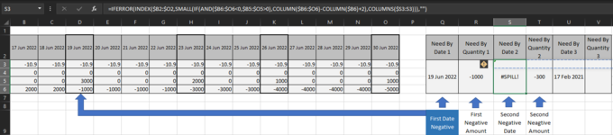
Here's how my sheet is laid out. Highlights are there for demonstration purposes only, but the pinkish area contains the cells in which I want the magic to occur.
Row 1 is dedicated to column headers, which are actually names of elements users are being evaluated upon ("did they do this?"). Rows 2-6 are the answers for each user (the user name is entered in column A). So Column A is the list of names, Columns B-K are the answers (yes / no / N/A)
The sample below gives a visual. The red text (in First Instance/Second Instance columns) show what I want to appear. The black text a couple of rows down shows the result from my testing (explained next paragraph).
During my time trying to figure it out myself, a basic index Match =INDEX($B$1:$E$1,MATCH("No",B4:E4,0) in F4 returned 'Question 1', but an attempt to expand upon that in F5 {=INDEX($B$1:$E$1,SMALL(IF($B4:$E4="No",COLUMN($B4:$E4)),2))} returned 'Question 3', which is of course is incorrect.
Thank you for any assistance you can provide.
<colgroup><col width="120" style="width: 90pt; mso-width-source: userset; mso-width-alt: 4388;" span="10">
<tbody>
</tbody>
I've searched and searched, without finding exactly what I'm looking for. My goal in this exercise is to look horizontally across an array, find the Nth occurrence of a specific text string ("No") and then, in the appropriate cell, return a value that is the column header for the column in which that string occurred. In the next cell on the same row, it would return the next occurrence's column header.
Here's how my sheet is laid out. Highlights are there for demonstration purposes only, but the pinkish area contains the cells in which I want the magic to occur.
Row 1 is dedicated to column headers, which are actually names of elements users are being evaluated upon ("did they do this?"). Rows 2-6 are the answers for each user (the user name is entered in column A). So Column A is the list of names, Columns B-K are the answers (yes / no / N/A)
The sample below gives a visual. The red text (in First Instance/Second Instance columns) show what I want to appear. The black text a couple of rows down shows the result from my testing (explained next paragraph).
During my time trying to figure it out myself, a basic index Match =INDEX($B$1:$E$1,MATCH("No",B4:E4,0) in F4 returned 'Question 1', but an attempt to expand upon that in F5 {=INDEX($B$1:$E$1,SMALL(IF($B4:$E4="No",COLUMN($B4:$E4)),2))} returned 'Question 3', which is of course is incorrect.
Thank you for any assistance you can provide.
| A | B | C | D | E | F | G | H | I | J | |
| 1 | Agent Name | Question 1 | Question 2 | Question 3 | Question 4 | First Instance | Second Instance | Third Instance | 4th Instance | 5th Instance |
| 2 | Bill | Yes | Yes | No | No | Question 3 | Question 4 | |||
| 3 | Ben | Yes | Yes | Yes | Yes | |||||
| 4 | Mary | No | No | Yes | Yes | Question 1 | Question 3 | |||
| 5 | Betty | Yes | Yes | Yes | Yes | |||||
| 6 | Sonya | No | No | Yes | Yes | Question 1 | Question 2 |
") I put it in my actual worksheet and it works perfectly (not that I had any doubt, of course).
I put it in my actual worksheet and it works perfectly (not that I had any doubt, of course).