Hi All !
First post here, but have found solutions on this board to 100s of problems over the years. Thank you all, very, very much!
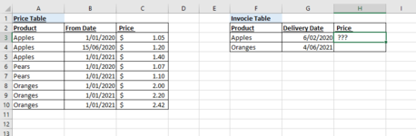
I need to find the price of a product based on the delivery date and product name.

I think it can be done with SUMIFS, but I'll have to add a "Price To" date. Additionally, I think, I may also have to divide by COUNTIFS to allow for an error/double-up in the price table?
works great but only returns the dates, not the corresponding price...
The data is not sorted and array formulas are not an option, because they are difficult to understand by the multiple users (including me). Any thoughts....?
For those of you who came across this post looking to solve a similar problem, the below may be helpful:

 www.mrexcel.com
www.mrexcel.com
www.mrexcel.com
P.S. The above is an example, I don't have any fruit to sell!
First post here, but have found solutions on this board to 100s of problems over the years. Thank you all, very, very much!
I need to find the price of a product based on the delivery date and product name.
I think it can be done with SUMIFS, but I'll have to add a "Price To" date. Additionally, I think, I may also have to divide by COUNTIFS to allow for an error/double-up in the price table?
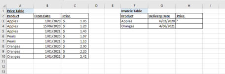
Excel Formula:
=MAXIFS(B3:B10, B3:B10, "<="&G3)The data is not sorted and array formulas are not an option, because they are difficult to understand by the multiple users (including me). Any thoughts....?
For those of you who came across this post looking to solve a similar problem, the below may be helpful:
Summing for Date Ranges
Hello Excel Guru's, I cant seem to sum the costs associated with these date ranges. Grateful for your assistance. thank you in advance. There are 2 sheets. Please scroll down for the date ranges. I have this in one sheet: 1/2/2020 11/29/2030 1/31/2026 1/31/2046 $ 2.00 $...
How to obtain MAXIF VALUE and it's corresponding cell?
A 27/06/2018 B Deadlift C 1 D 50 E 8 27/06/2018 Deadlift 2 110 5 27/06/2018 Deadlift 3 130 5 27/06/2018 Deadlift 4 130 4 27/06/2018 Deadlift 5 120 5 28/06/2018 Lat Pulldown 1 50 10 28/06/2018 Lat Pulldown 2 50 10 28/06/2018 Lat Pulldown 3 55 7 28/06/2018 Lat Pulldown 4 50 9...
P.S. The above is an example, I don't have any fruit to sell!