FIND SUM OF MULTIPLE OUTPUT DATA FOR SINGLE INPUT DATA UNTIL NEXT INPUT DATA IS FOUND

cclp

New Member
Joined
Jun 5, 2022
Messages
4
Office Version
  1. 365
  2. 2021
  3. 2016
Platform
  1. Windows
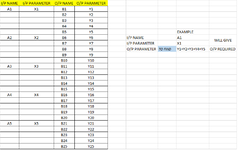
My query is regarding MS Excel. Please refer below image for better understanding. I have one input data and it parameter, for which I get multiple output data and their respective parameters. I need to build a table where I feed the input data and receive a sum of output data parameters.
 

Attachments

  • excel doubt.png
    excel doubt.png
    20.4 KB · Views: 8

Excel Facts

How to create a cell-sized chart?
Tiny charts, called Sparklines, were added to Excel 2010. Look for Sparklines on the Insert tab.
cannot manipulate data in a picture. Please reload your sample data using XL2BB. See my signature.
 
Upvote 0
Based on what you've described, something like this should give you the sum, but you should consider flattening your table to avoid the difficulties in determining where the range to sum begins and ends.
MrExcel_20220603.xlsx
ABCDEFGH
1
2A1X11
32colAA2
43colBX2
54sum of D26
6A2X25
76
87
98
10A3X39
1110
1211
13somethingsomething12
1413
1514
1615
17xx
Sheet8
Cell Formulas
RangeFormula
H5H5=LET(seq,ROW(A$2:A$100)-ROW(A$2)+1,cidx,FILTER(seq,(A$2:A$100<>"")*(B$2:B$100<>"")),sidx,FILTER(seq,(A$2:A$100=$H$3)*(B$2:B$100=H4)),eidx,INDEX(cidx,MATCH(sidx,cidx,0)+1),SUM(FILTER(D$2:D$100,(seq>=sidx)*(seq<eidx))))

If you flattened the table so that it appears like this, then the summation can be done with a much simpler approach:
MrExcel_20220603.xlsx
JKLMNOPQ
1
2A1X11
3A1X12colAA2
4A1X13colBX2
5A1X14sum of D26
6A2X25
7A2X26
8A2X27
9A2X28
10A3X39
11A3X310
12A3X311
13somethingsomething12
14somethingsomething13
15somethingsomething14
16somethingsomething15
17xx
Sheet8
Cell Formulas
RangeFormula
J3:K5,J14:K16,J11:K12,J7:K9J3=J2
Q5Q5=SUMIFS(M$2:M$100,J$2:J$100,$Q$3,K$2:K$100,$Q$4)

To flatten the table, you could use a VBA script to fill in the blanks, Power Query, or even the approach described in the 1st method here (which is what I used).

Thanks for replying
How will the formula modify if we don't need column B, Just Column A and Sum of corresponding elements in Column D
 
Upvote 0
The "without B" version is shown in H6 and Q6:
MrExcel_20220603.xlsx
ABCDEFGHIJKLMNOPQ
1
2A1X11A1X1x11
32colAA2A1X12colAA2
43colBX2A1X13colBX2
54sum of D26A1X14sum of D26
6A2X25sum of D (w/o B)26A2X2x25sum of D (w/o B)26
76A2X26
87A2X27
98A2X28
10A3X39A3X3x39
1110A3X310
1211A3X311
13somethingsomething12somethingsomething12
1413somethingsomething13
1514somethingsomething14
1615somethingsomething15
17xxxx
Sheet8
Cell Formulas
RangeFormula
J3:K5,J14:K16,J11:K12,J7:K9J3=J2
H5H5=LET(seq,ROW(A$2:A$100)-ROW(A$2)+1,cidx,FILTER(seq,(A$2:A$100<>"")*(B$2:B$100<>"")),sidx,FILTER(seq,(A$2:A$100=$H$3)*(B$2:B$100=H4)),eidx,INDEX(cidx,MATCH(sidx,cidx,0)+1),SUM(FILTER(D$2:D$100,(seq>=sidx)*(seq<eidx))))
H6H6=LET(seq,ROW(A$2:A$100)-ROW(A$2)+1,cidx,FILTER(seq,A$2:A$100<>""),sidx,FILTER(seq,A$2:A$100=$H$3),eidx,INDEX(cidx,MATCH(sidx,cidx,0)+1),SUM(FILTER(D$2:D$100,(seq>=sidx)*(seq<eidx))))
Q5Q5=SUMIFS(M$2:M$100,J$2:J$100,$Q$3,K$2:K$100,$Q$4)
Q6Q6=SUMIFS(M$2:M$100,J$2:J$100,$Q$3)
Thanks for your help!!
 
Upvote 0

Forum statistics

Threads
1,214,915
Messages
6,122,217
Members
449,074
Latest member
cancansova

We've detected that you are using an adblocker.

We have a great community of people providing Excel help here, but the hosting costs are enormous. You can help keep this site running by allowing ads on MrExcel.com.
Allow Ads at MrExcel

Which adblocker are you using?

Disable AdBlock

Follow these easy steps to disable AdBlock

1)Click on the icon in the browser’s toolbar.
2)Click on the icon in the browser’s toolbar.
2)Click on the "Pause on this site" option.
Go back

Disable AdBlock Plus

Follow these easy steps to disable AdBlock Plus

1)Click on the icon in the browser’s toolbar.
2)Click on the toggle to disable it for "mrexcel.com".
Go back

Disable uBlock Origin

Follow these easy steps to disable uBlock Origin

1)Click on the icon in the browser’s toolbar.
2)Click on the "Power" button.
3)Click on the "Refresh" button.
Go back

Disable uBlock

Follow these easy steps to disable uBlock

1)Click on the icon in the browser’s toolbar.
2)Click on the "Power" button.
3)Click on the "Refresh" button.
Go back
Back
Top