Find the partial text in string and then find matching minimum price from multiple options

[mljohn]

I am trying to find the minimum price that matches the partial string.
I have several suppliers with the same part number with different pricing.

There are several matching part numbers for the same item. Each item has a list of part numbers. Some vendors show a more complete list of the part numbers for each item than others.
Example: TN450
Example: TN750
Example: TN221BK, TN225BK
Example: 6497B001, 6514B001, 6515B001, 6516B001

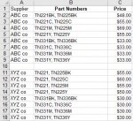
The supplier name for the parts is in Col A.
My part numbers are in a separate sheet "PartandPrice" in Col B.
My prices for those part numbers are in the same sheet "PartandPrice" in Col C.

I have tried the formula in Sheet4 =IF(A1<>"",INDEX(PartandPrice!C:C,INDEX(MATCH("*"&A1&",*",PartandPrice!B:B&",",0),)),"") to find the partial item and it seems to work.
However, since I have a list of multiple supplier lists with similar part numbers it does not work to find the minimum price amongst the various suppliers.


I would like to enter in sheet4 A1 the part number "TN336C" and in B1 get the price "$30.00" and also have C1 show which supplier that price came from.
The formula would go to the "PartandPrice" sheet and find the matching "TN336C" from the list of part numbers and find the lowest price and enter it into B1 and show which supplier that came from in D1

See the Image.

 

[jasonb75]

To find the price

=IF(A1="","",MINIFS(PartandPrice!C:C,PartandPrice!B:B,"*"&A1&"*"))

To find the supplier, note that other than the first index range, this formula should not be used with full columns. It either needs to be set to a sensible number of rows, or use dynamic ranges.

=IFERROR(INDEX(PartandPrice!A:A,AGGREGATE(15,6,ROW(PartandPrice!$A$2:$A$100)/ISNUMBER(SEARCH(A1,PartandPrice!$B$2:$B$100))/(PartandPrice!$C$2:$C$200=B1),1),"")

 

[KRice]

Hi Jason,
I think something may not have copied over correctly...at the end of the supplier formula, another right parenthesis is needed after the 1, if I'm not mistaken.
=IFERROR(INDEX(PartandPrice!A:A,AGGREGATE(15,6,ROW(PartandPrice!$A$2:$A$100)/ISNUMBER(SEARCH(A1,PartandPrice!$B$2:$B$100))/(PartandPrice!$C$2:$C$200=B1),1)),"")

 

[jasonb75]

I think something may not have copied over correctly...

Thanks for correcting that, Kirk. There was no copyable sample so I just typed the formula out here, usually have too many parenthesis in the array

 

[mljohn]

You guys are fantastic. This worked perfectly!