Finding % based on conditional format dates

gulonraid

New Member
Joined
Apr 13, 2016
Messages
12
Good morning,

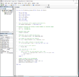
I am building a training tracker for work. I figured out how to use the conditional formatting to highlight when training will be due based on expiration dates. What I would like to do it have it show a % next to a persons name based on their row of training. So if a CBT date goes red, it would lower the %. I have attached the excel doc to show what it currently looks like.
Tracker_Snippit.PNG
 

Excel Facts

Wildcard in VLOOKUP
Use =VLOOKUP("Apple*" to find apple, Apple, or applesauce
You would not base your formulas on the Conditional Formatting (Excel formulas only run off of values, not on formatting).
However, you may be able to use the same conditions/rules you used for Conditional Formatting in your formulas.
(Since you have not told us what those Conditional Formatting rules are, we cannot say for certain).
 
Upvote 0
Joe4 please see below minisheet. All conditional formatting is based on either blanks, or based on less then =TODAY()-365, etc to match the dates with the expiration timeframe.

Training Tracker.xlsx
ABCDEFGHIJKLMNO
1Training 1Training 2Training 3Training 4Training 5Training 6Training 7Training 8Training 9Training 10Training 11Training 12
2Percent Complete0%
3Good forMonths0361236362412183603648
4PersonPercent Comp.
5Name 10%22-Oct-201919-Mar-20209-Dec-202117-Aug-201817-Aug-201824-Jan-201918-May-202113-Mar-201912-Sep-201818-May-202031-Jul-2020
6Name 20%15-Jan-201713-Jan-20216-Oct-202121-Aug-202029-Sep-202015-Nov-202129-Nov-202018-May-201726-Sep-201812-Jan-202126-Nov-2017
7Name 30%15-Nov-20216-Oct-20217-Oct-20217-Oct-202113-Aug-202115-Nov-202115-Nov-20217-Oct-2021
8Name 40%2-Sep-201927-Mar-202019-Mar-202116-Oct-201916-Oct-201913-Dec-201931-Jul-202127-Jan-19003-Nov-201925-Nov-202027-Mar-2020
9Name 50%13-Aug-2021
10Name 60%6-Oct-20217-Oct-202113-Aug-20217-Oct-2021
11Name 70%13-Aug-202118-Nov-202113-Aug-2021
12Name 80%5-Nov-20219-Dec-202122-Nov-202122-Nov-202113-Aug-202122-Nov-202122-Nov-202122-Nov-202122-Nov-2021
13Name 90%17-Jan-20146-Jun-20199-Dec-20212-Mar-20152-Mar-20158-Jun-202013-Jan-202116-Jan-201710-Sep-201817-Jul-201918-Aug-2016
14Name 100%6-Apr-201926-Jan-202118-Dec-201921-Aug-20204-Jun-202018-Dec-201931-Dec-202018-Jun-202016-May-201920-Jan-202113-Sep-2019
15Name 110%25-Mar-20159-Dec-20216-Oct-20219-Dec-20219-Dec-20219-Mar-202110-Jan-20219-Dec-202112-Apr-201812-Apr-2019
16Name 120%22-Nov-20216-Oct-20217-Oct-20217-Oct-202113-Aug-20217-Oct-202122-Nov-202110-Dec-20217-Oct-2021
17Name 130%10-Oct-20206-Oct-20207-Dec-20216-Oct-20206-Oct-202016-Apr-201924-Sep-202131-Mar-202030-Sep-201820-Jul-20177-May-2017
18Name 140%7-Dec-202118-Nov-2021
19Name 150%11-Nov-201618-Nov-20217-Dec-202115-Feb-201718-Nov-202122-Jul-20208-Jan-202122-Jul-20209-Aug-201820-Dec-20171-Sep-2017
20Name 160%25-Aug-20147-Feb-20197-Dec-202122-May-202022-May-202015-Nov-202127-May-202118-Jun-20203-Apr-201825-Nov-20203-Oct-2020
21Name 170%8-Feb-201614-Dec-20207-Dec-202122-Jul-20205-Oct-202018-Nov-20211-Oct-20212-Dec-202024-Jan-201820-Jan-202113-Feb-2018
22Name 180%9-Dec-20219-Dec-202018-Nov-20213-Jun-20219-Dec-202022-Oct-20209-Dec-2020
23Name 190%10-Jan-201812-Nov-20216-Oct-20217-Oct-20217-Oct-202115-Nov-202110-Nov-20207-Oct-202120-Dec-201812-Nov-202111-Jan-2018
24Name 200%3-Jun-20206-Oct-202125-Sep-201828-May-201826-Jan-20196-Jul-202123-Jan-201920-Jun-201922-Jul-201928-May-2018
25Name 210%23-Jul-202120-Nov-20218-Aug-20217-Oct-20217-Oct-202110-Dec-202013-Aug-20217-Oct-202120-Nov-202120-Nov-202120-Nov-2021
26Name 220%16-Dec-201920-Jun-20208-Aug-202117-Dec-20196-Dec-20209-Mar-20217-Dec-20206-Dec-202022-Dec-201924-Feb-202020-Dec-2019
27Name 230%1-Oct-201927-Sep-201818-Dec-20194-Dec-20204-Dec-202015-Nov-202112-Jun-202118-Jun-202022-Jan-201825-Jan-20161-Jul-2017
28Name 240%23-Dec-201910-Dec-20216-Oct-202124-Feb-201924-Feb-201911-Dec-202027-Dec-20208-May-202031-May-201910-Dec-202122-Feb-2019
29Name 250%12-Dec-202112-Dec-20219-Dec-202112-Dec-202113-Aug-202112-Dec-202112-Dec-202112-Dec-202112-Dec-2021
Sheet1
Cell Formulas
RangeFormula
B2B2=SUM(B5:B63)/59
Cells with Conditional Formatting
CellConditionCell FormatStop If True
X5:X63,S5:T63,O5:Q63Cell Value<TODAY()-1460textNO
X5:X63,S5:T63,O5:Q63Cell Valuebetween TODAY()-1415 and TODAY()-1560textNO
X5:X63,S5:T63,O5:Q63Cell Value<TODAY()+1textNO
E5:E63,G5:H63,L5:L63,N5:N63,AB5:AC63,AH5:AH63,AK5:AN63Cell Value<TODAY()-1095textNO
E5:E63,G5:H63,L5:L63,N5:N63,AB5:AC63,AH5:AH63,AK5:AN63Cell Valuebetween TODAY()-1050 and TODAY()-1095textNO
E5:E63,G5:H63,L5:L63,N5:N63,AB5:AC63,AH5:AH63,AK5:AN63Cell Value<TODAY()+1textNO
AF5:AF63,AD5:AD63,Y5:Y63,I5:I63Cell Value<TODAY()-730textNO
F5:F63,J5:J63,R5:R63,U5:U63,Z5:Z63,AE5:AE63Cell Value<TODAY()-365textNO
F5:F63,J5:J63,R5:R63,U5:U63,Z5:Z63,AE5:AE63Cell Valuebetween TODAY()-365 and TODAY()-320textNO
AO5:AP63,AA5:AA63,V5:W63,K5:K63Cell Value<TODAY()-547textNO
AO5:AP63,AA5:AA63,V5:W63,K5:K63Cell Valuebetween TODAY()-547 and TODAY()-502textNO
AO5:AP63,AA5:AA63,V5:W63,K5:K63Cell Value<TODAY()+1textNO
AD5:AF63,Y5:Y63,I5:I63Cell Valuebetween TODAY()-685 and TODAY()-730textNO
AD5:AF63,Y5:Y63,I5:I63Cell Value<TODAY()+1textNO
F5:F63,J5:J63,R5:R63,U5:U63,Z5:Z63,AE5:AE63Cell Value<TODAY()+1textNO
D5:D63,M5:M63,AG5:AG63,AI5:AJ63Celldoes not contain a blank value textNO
D5:AQ63Cellcontains a blank value textNO
B2,B5:B63Cell Value>0.9textNO
B2,B5:B63Cell Valuebetween 0.75 and 0.9textNO
B2,B5:B63Cell Valuebetween 0 and 0.75textNO
A5:A63Expression=#REF!="1"textNO
 
Upvote 0
OK, can you pick a row, and walk me through an example of what should happen, explaining the logic behind it?
 
Upvote 0
Of course. I can use row 5 as the example..

Each column starting a D5 has a date that shows when the team member completed the training. For instance E6, the training is good for 36 months so the conditional formatting is set to when it hits 45 days prior to the 36 month mark, it will turn yellow and once it passes the 36 month mark it turns red. What I would like to do if it is possible is be able to track a total percentage based on how many of the trainings are completed.

In the mini sheet it goes from Training 1 to Training 12. Name 5 (row 5) has good dates for 7/12 trainings. Is it possible to show a % in B5 based on those conditional formatting so that the percentage as of now would show 58%, but if more of the dates turned green or red would change that percentage? Please let me know if this makes sense.
 
Upvote 0
OK, since you have at least 6 different month possibilities (0, 12, 18, 24, 36, 48), that formula could be quite complex, because you would have to account for each one, unless you can build some sort of rule that uses the months dynamically in your rules.

I might come at this a different way. While you cannot use native Excel formulas to count cells colored by Conditional Formatting, you CAN use VBA to do so.
Here is a link that shows you how to do that: ExcelSirJi | VBA Code to Count Color Cells with Conditional Formatting

If you aren't sure what color codes your pink, green, and yellow colors are, you can get them easily by selecting one of those cells, and then running this VBA code:
VBA Code:
Sub GetColor()
    MsgBox ActiveCell.DisplayFormat.Interior.Color
End Sub

So if you get the code for the "green" color (which I think is what you are trying to count), you could use that in the code.

I would probably do this in a Worksheet_Change event procedure. As dates are manually added to the body of your data, you can have VBA code automatically fire off that updates the formula in column B of that row.

If you need help in doing that, please run the code I posted above to get the color code for the green cells and post it here, and let me know what the last column is that dates will be entered into.
 
Upvote 0
I came up with some VBA code that I think will do what you want.
You just need to be sure to put it in the Worksheet module for the sheet that you want to apply it to, and make the edits, where needed.

So the code looks like this:
VBA Code:
Private Sub Worksheet_Change(ByVal Target As Range)

    Dim sc As Long
    Dim ec As Long
    Dim ccode As Double
    Dim lr As Long
    Dim rng As Range
    Dim r As Long
    Dim c As Long
    Dim ctr As Long
    
'   Exit if multiple cells updated simultaneously
    If Target.CountLarge > 1 Then Exit Sub

'***Specify starting and ending column numbers in watched range
    sc = 4  '(column D)
    ec = 15 '(column O)
    
'***Specify color code
    ccode = 10285055
    
'   Find last row in column A with data
    lr = Cells(Rows.Count, "A").End(xlUp).Row
    
'   Set range to check for new entries
    Set rng = Range(Cells(5, sc), Cells(lr, ec))
    
'   Exit if no cells updated in watched range
    If Intersect(Target, rng) Is Nothing Then Exit Sub
    
'   Get row of cells just updates
    r = Target.Row
    
'   Loop through row to get count
    For c = sc To ec
'       Add to counter if cell matches color code
        If Cells(r, c).DisplayFormat.Interior.Color = ccode Then
            ctr = ctr + 1
        End If
    Next c
    
'   Update column B with percentage
    Application.EnableEvents = False
    Cells(r, "B").Value = ctr / (ec - sc + 1)
    Application.EnableEvents = True
    
End Sub
and the values you would need to change/edit to match your scenario are the ones highlighted below in red:
Rich (BB code):
'***Specify starting and ending column numbers in watched range
    sc = 4  '(column D)
    ec = 15 '(column O)
    
'***Specify color code
    ccode = 10285055
Assuming that you have placed the code in the proper sheet module, the code will run automatically as you manually enter/edit dates in the body of the table.
 
Upvote 0
Should it pull a Macro after inputting the VBA and changing the values to ec = 43 '(column AQ) and changing the color code?
 
Upvote 0
Should it pull a Macro after inputting the VBA and changing the values to ec = 43 '(column AQ) and changing the color code?
I am not sure what you mean/what you are asking.
Note in Excel, VBA and Macros are really the same thing.

In order for this code to run automatically, it MUST be placed in the proper sheet module.
One way to ensure that is to go to the page that you want to apply it to, right-click on the Sheet tab name at the bottom of the screeen, select "View Code", and copy/paste the VBA code in the VB Editor window that pops up.

You also CANNOT change the first line of the code. It MUST look exactly like:
VBA Code:
Private Sub Worksheet_Change(ByVal Target As Range)
in order to run automatically when a cell is manually changed on that sheet.
 
Upvote 0
I have attached a screenshot of the code. Should it automatically fill the % out in B5 and down?
 

Attachments

  • vba_snippit.PNG
    vba_snippit.PNG
    89.7 KB · Views: 7
Upvote 0

Forum statistics

Threads
1,214,923
Messages
6,122,289
Members
449,077
Latest member
Rkmenon

We've detected that you are using an adblocker.

We have a great community of people providing Excel help here, but the hosting costs are enormous. You can help keep this site running by allowing ads on MrExcel.com.
Allow Ads at MrExcel

Which adblocker are you using?

Disable AdBlock

Follow these easy steps to disable AdBlock

1)Click on the icon in the browser’s toolbar.
2)Click on the icon in the browser’s toolbar.
2)Click on the "Pause on this site" option.
Go back

Disable AdBlock Plus

Follow these easy steps to disable AdBlock Plus

1)Click on the icon in the browser’s toolbar.
2)Click on the toggle to disable it for "mrexcel.com".
Go back

Disable uBlock Origin

Follow these easy steps to disable uBlock Origin

1)Click on the icon in the browser’s toolbar.
2)Click on the "Power" button.
3)Click on the "Refresh" button.
Go back

Disable uBlock

Follow these easy steps to disable uBlock

1)Click on the icon in the browser’s toolbar.
2)Click on the "Power" button.
3)Click on the "Refresh" button.
Go back
Back
Top