Finding bottom minimum values

[bbran19]

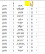
I use this formula to assign A,B,C,D to the highest value, next highest and so on in Column H based on a list as attached using column C and D as differentiators.

=IF($H2=MAX(($C$2:$C$299=$C2)*($D$2:$D$299=$D2)*($H$2:$H$299)),"A",IF(H2=LARGE(($D$2:$D$299=$D2)*($H$2:$H$299)*($C$2:$C$299=$C2),2),"B",IF(H2=LARGE(($D$2:$D$299=$D2)*($H$2:$H$299)*($C$2:$C$299=$C2),3),"C",IF(H2=LARGE(($D$2:$D$299=$D2)*($H$2:$H$299)*($C$2:$C$299=$C2),4),"D",""))))

But I can not for the life of me workout how to assign A,B,C,D to find the Lowest value, next lowest, and so on in another column.

 

[Peter_SSs]

Is it possible to modify the formule to recognise two columns Track (column A) and Race Number (Column B) and then reference Column E to show A,B,C,D in Column F based on A being the highest value, B the next highest etc.

Sure ..

21 05 24.xlsm
	A	B	C	D	E	F
1	Track	RACE	No	Name	Rating	Perf Stats
2	Taree	1	1	Adamdeeant	60.5
3	Taree	1	2	Bangalley Lad	68.0
4	Taree	1	3	Neretva	70.3	D
5	Taree	1	4	Sophie's Lass	81.1	C
6	Taree	1	5	Bay Of Bengal	116.7	A
7	Taree	1	6	Crowned Empress	100.4	B
8	Taree	1	8	No Dreams All Hope	46.5
9	Taree	1	9	Budawang	30.0
10	Albury	2	1	Smuggler's Bay	143.1	A
11	Albury	2	2	Native Leaf	60.4	D
12	Albury	2	3	Redneck Princess	81.7	C
13	Albury	2	4	Sunshine Moshe	47.9
14	Albury	2	5	Kokomo Bliss	54.5
15	Albury	2	6	Miss Elsie May	82.9	B
16	Albury	2	7	Money In Mud	45.3
17	Albury	2	8	On The Bell	32.1
18	Albury	2	11	Master Knight	33.7
19	Albury	2	12	Congenial Mistress	26.6
20	Albury	2	13	All The Wine	31.1
21	Albury	3	3	I'm The Business	61.2	D
22	Albury	3	4	Dubai Centre	57.9
23	Albury	3	5	Electric Storm	53.3
24	Albury	3	6	Sizzling Cat	88.7	B
25	Albury	3	7	Elope To Vegas	91.4	A
26	Albury	3	8	Kentucky Dream	67.5	C
27	Albury	3	9	The Chaplain	52.7
28	Albury	3	10	Zoey Lass	31.6
29	Albury	3	11	Cape Cluster	31.9
30	Albury	3	12	Sun Master	34.2
31	Albury	3	13	Georgian Court	33.9
ABCD

Cell Formulas
Range	Formula
F2:F31	F2	=MID("ABCD",MATCH(E2,SORT(FILTER(E$2:E$100,(A$2:A$100=A2)*(B$2:B$100=B2)),,-1),0),1)