Finding the Highest Letter in 2 Separate Cells, A has to be above NC?

[jameslaz63]

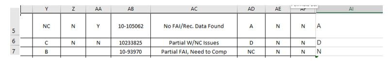
Hi and thank you in advance for any assistance provided. I am trying to create a formula to pick the high of 2 letters in 2 separate cells (A5 and AB5). I found your answer to another question that led me to "=IF(COUNT(Y5,AD5),MAX(Y5,AD5),CHAR(MAX(IF(ISTEXT(Y5,AD5),CODE(Y5,AD5)))))" and that works great. My problem is I have the letters NC, A, B, C and D and NC is the lowest and D is the highest (NC, A, B, C. D). For my NC cless it returns N as the higher letter of cores. Any ideas on how to make the NC the lowers letter in my list?

Thank you,
James

 

[jameslaz63]

My bad, the formula I put is not quite right, help on that is appreciated as well. .