Finding which 4 boxes can hold product X's dimensions

[mystic_muffin]

Hey, Friends;

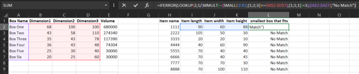
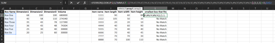
So lets say I have 4 box sizes with their dimension in a list. I also have an array of objects to fit in the boxes with their own dimensions. I only want to fit one item in one box so i want the box that fits the item the best. Under my "box that fits" column, I'd like a formula or something that can look down the item dimensions and compare them to the box dimensions and find whatever box works best with item, then display the name from column A. So if i have an item that 9x9x9 and a box that is 10x10x10, my sheet will choose that box because the item is just less than the box size.

box name	box length	box width	box height	item name	item length	item width	item height	box that fits
box one	100	68	100	1111	90	60	88
box two	110	58	43	2222	105	50	30
box three	78	43	35	3333	20	20	10
box four	48	43	36	4444	40	60	90

<tbody>
</tbody>

Can anyone help me out with this?

I appreciate any assistance. Let me know if i need to clear anything up.

 

[Eric W]

For ease of visualization, I split the tables like so:

	A	B	C	D	E
1	box name	box length	box width	box height
2	box one	100	68	100
3	box two	110	58	43
4	box three	78	43	35
5	box four	48	43	36
6
7
8	item name	item length	item width	item height	smallest box that fits
9	1111	90	60	88	box one
10	2222	105	50	30	box two
11	3333	20	20	10	box four
12	4444	40	60	90	box one
13	5555	70	40	40	box two
14	6666	70	40	45	box one
15	7777	70	70	30	No Match
16

<tbody>
</tbody>

Sheet8​

Array Formulas Cell Formula E9 {=IFERROR(INDEX($A$2:$A$5,MOD(SMALL(IF(D9<=$D$2:$D$5,IF(MAX(B9,C9)<=$B$2:$B$5,IF(MIN(B9,C9)<=$C$2:$C$5,$B$2:$B$5*$C$2:$C$5+(ROW($A$2:$A$5)-ROW($A$2)+1)/100))),1),1)*100),"No Match")} <tbody> </tbody> Entered with Ctrl+Shift+Enter. If entered correctly, Excel will surround with curly braces {}. Note: Do not try and enter the {} manually yourself

<tbody>
</tbody>

I made a few assumptions. First, that on the first table, the length is always more than the width. Second, on the second table, the length and width can be in either order, and that it doesn't matter which comes first, since you can rotate the item 90 degrees. The height is pretty much required, since most products have a definite top/bottom. And for smallest box, I chose the box with the smallest square inches for the base, that both length and width dimensions fit, and the height fits.

Given that, the array formula in E9 should get you what you want. Let me know what you think.

 

[mystic_muffin]

For ease of visualization, I split the tables like so:

	A	B	C	D	E
1	box name	box length	box width	box height
2	box one	100	68	100
3	box two	110	58	43
4	box three	78	43	35
5	box four	48	43	36
6
7
8	item name	item length	item width	item height	smallest box that fits
9	1111	90	60	88	box one
10	2222	105	50	30	box two
11	3333	20	20	10	box four
12	4444	40	60	90	box one
13	5555	70	40	40	box two
14	6666	70	40	45	box one
15	7777	70	70	30	No Match
16

<tbody>
</tbody>

Sheet8​

Array Formulas Cell Formula E9 {=IFERROR(INDEX($A$2:$A$5,MOD(SMALL(IF(D9<=$D$2:$D$5,IF(MAX(B9,C9)<=$B$2:$B$5,IF(MIN(B9,C9)<=$C$2:$C$5,$B$2:$B$5*$C$2:$C$5+(ROW($A$2:$A$5)-ROW($A$2)+1)/100))),1),1)*100),"No Match")} <tbody> </tbody> Entered with Ctrl+Shift+Enter. If entered correctly, Excel will surround with curly braces {}. Note: Do not try and enter the {} manually yourself

<tbody>
</tbody>

I made a few assumptions. First, that on the first table, the length is always more than the width. Second, on the second table, the length and width can be in either order, and that it doesn't matter which comes first, since you can rotate the item 90 degrees. The height is pretty much required, since most products have a definite top/bottom. And for smallest box, I chose the box with the smallest square inches for the base, that both length and width dimensions fit, and the height fits.

Given that, the array formula in E9 should get you what you want. Let me know what you think.

Works wonderfully! This is exactly what I was looking for. Thank so much, i really appreciate it. Now I need to fiddle around with it so i can learn how this thing works!

 

[Marcelo Branco]

If the sizes of the boxes are in descending order, maybe this formula also works (using data sample provided by Eric in post #2 )

Formula in E9 copied down
=IFERROR(LOOKUP(2,1/(MMULT(--($B$2:$D$5-B9:D9>0),{1;1;1})=3),$A$2:$A$5),"No Match")
confirmed with just Enter

M.

 

[mystic_muffin]

Let me know what you think.

Now that I've goofed around with this some, one thing:

If I paint this formula down a column where there is no dimension info in a row yet, it assumes the dimensions are '0' and it assumes it will fit in the smallest box.

Is there any way that we can stop the formula from calculating if there is a '0'?

Or is there a more eloquent way of doing this?

I appreciate the help!

 

[Eric W]

It's easy enough to add a check to see if there's an Item Name before calculating:

	A	B	C	D	E	F	G
1	box name	box length	box width	box height
2	Box one	100	68	100
3	Box two	110	58	43
4	Box three	78	43	35
5	Box Four	48	43	36
6
7
8	Item name	item length	item width	Item height	Smallest box that fits
9	1111	90	60	88	Box one		Box one
10	2222	105	50	30	Box two		Box two
11	3333	20	20	10	Box Four		Box Four
12	4444	40	60	90	Box one		Box one
13	5555	70	40	40	Box two		Box two
14	6666	70	40	45	Box one		Box one
15	7777	70	70	30	No Match		No Match
16	8888	50	105	30	Box two		No Match
17

<colgroup><col style="width: 25pxpx"><col><col><col><col><col><col><col></colgroup><thead>
</thead><tbody>
</tbody>

Sheet11​

Worksheet Formulas Cell Formula G9 =IF(A9="","",IFERROR(LOOKUP(2,1/(MMULT(--($B$2:$D$5-B9:D9>0),{1;1;1})=3),$A$2:$A$5),"No Match")) <thead> </thead><tbody> </tbody>

<tbody>
</tbody>

Array Formulas Cell Formula E9 {=IF(A9="","",IFERROR(INDEX($A$2:$A$5,MOD(SMALL(IF(D9<=$D$2:$D$5,IF(MAX(B9,C9)<=$B$2:$B$5,IF(MIN(B9,C9)<=$C$2:$C$5,$B$2:$B$5*$C$2:$C$5+(ROW($A$2:$A$5)-ROW($A$2)+1)/100))),1),1)*100),"No Match"))} <thead> </thead><tbody> </tbody> Entered with Ctrl+Shift+Enter. If entered correctly, Excel will surround with curly braces {}. Note: Do not try and enter the {} manually yourself

<tbody>
</tbody>

I added Marcelo's formula as well, with the same change. His seems to work just as well, and is shorter, although I haven't tested it extensively. The one difference is that his requires you to enter the largest dimension first in the second table, to match the first table, as well as having table 1 in descending box size. Items 2222 and 8888 are the same with just the height and width reversed.

 

[Marcelo Branco]

My formula above needs a small adjustment
=IFERROR(LOOKUP(2,1/(MMULT(--($B$2:$D$5-B9:D9>=0),{1;1;1})=3),$A$2:$A$5),"No Match")

M.

 

[Manu9211]

Hi all,

It's easy enough to add a check to see if there's an Item Name before calculating:

	A	B	C	D	E	F	G
1	box name	box length	box width	box height
2	Box one	100	68	100
3	Box two	110	58	43
4	Box three	78	43	35
5	Box Four	48	43	36
6
7
8	Item name	item length	item width	Item height	Smallest box that fits
9	1111	90	60	88	Box one		Box one
10	2222	105	50	30	Box two		Box two
11	3333	20	20	10	Box Four		Box Four
12	4444	40	60	90	Box one		Box one
13	5555	70	40	40	Box two		Box two
14	6666	70	40	45	Box one		Box one
15	7777	70	70	30	No Match		No Match
16	8888	50	105	30	Box two		No Match
17

<colgroup><col style="width: 25pxpx"><col><col><col><col><col><col><col></colgroup><thead>
</thead><tbody>
</tbody>

Sheet11​

Worksheet Formulas Cell Formula G9 =IF(A9="","",IFERROR(LOOKUP(2,1/(MMULT(--($B$2:$D$5-B9:D9>0),{1;1;1})=3),$A$2:$A$5),"No Match")) <thead> </thead><tbody> </tbody>

<tbody>
</tbody>

Array Formulas Cell Formula E9 {=IF(A9="","",IFERROR(INDEX($A$2:$A$5,MOD(SMALL(IF(D9<=$D$2:$D$5,IF(MAX(B9,C9)<=$B$2:$B$5,IF(MIN(B9,C9)<=$C$2:$C$5,$B$2:$B$5*$C$2:$C$5+(ROW($A$2:$A$5)-ROW($A$2)+1)/100))),1),1)*100),"No Match"))} <thead> </thead><tbody> </tbody> Entered with Ctrl+Shift+Enter. If entered correctly, Excel will surround with curly braces {}. Note: Do not try and enter the {} manually yourself

<tbody>
</tbody>



I added Marcelo's formula as well, with the same change. His seems to work just as well, and is shorter, although I haven't tested it extensively. The one difference is that his requires you to enter the largest dimension first in the second table, to match the first table, as well as having table 1 in descending box size. Items 2222 and 8888 are the same with just the height and width reversed.

the formula described above works great to solve the initial problem.

I would also like to consider not only turning the product 90 degrees to change length and width, but also turning the height dimension. Is there a way to modify the formula so that you can test if the product fits in the box by trying to rotate it in all dimensions? @Eric W

Thanks for your help

 

[Eric W]

Probably the easiest way is to use this variation of Marcelo's formula:

Book1 (version 1).xlsb
	A	B	C	D	E	F	G	H	I	J	K	L
1	Box Name	Dimension1	Dimension2	Dimension3	Volume			item name	item length	item width	item height	smallest box that fits
2	Box One	68	100	100	680000			1111	90	60	88	Box One
3	Box Two	43	58	110	274340			2222	105	50	30	Box Two
4	Box Three	35	43	78	117390			3333	20	20	10	Box Six
5	Box Four	36	43	48	74304			4444	40	60	90	Box One
6	Box Five	25	30	40	30000			5555	70	40	40	Box Two
7	Box Six	20	25	60	30000			6666	70	40	45	Box Two
8								7777	70	70	30	Box One
9								8888	70	100	110	No Match
Sheet6

Cell Formulas
Range	Formula
E2:E7	E2	=PRODUCT(B2:D2)
L2:L9	L2	=IFERROR(LOOKUP(2,1/(MMULT(--(SMALL(I2:K2,{1,2,3})<=$B$2:$D$7),{1;1;1})=3),$A$2:$A$7),"No Match")

To make this work right, the dimensions of the boxes in the A1:E7 table must be in order, smallest dimension on the left, largest on the right, then sort the rows of the tables in decreasing volume size. The dimensions in the H1:L9 table do not need to be entered in size order.

 

[Manu9211]

Probably the easiest way is to use this variation of Marcelo's formula:

Book1 (version 1).xlsb
	A	B	C	D	E	F	G	H	I	J	K	L
1	Box Name	Dimension1	Dimension2	Dimension3	Volume			item name	item length	item width	item height	smallest box that fits
2	Box One	68	100	100	680000			1111	90	60	88	Box One
3	Box Two	43	58	110	274340			2222	105	50	30	Box Two
4	Box Three	35	43	78	117390			3333	20	20	10	Box Six
5	Box Four	36	43	48	74304			4444	40	60	90	Box One
6	Box Five	25	30	40	30000			5555	70	40	40	Box Two
7	Box Six	20	25	60	30000			6666	70	40	45	Box Two
8								7777	70	70	30	Box One
9								8888	70	100	110	No Match
Sheet6

Cell Formulas
Range	Formula
E2:E7	E2	=PRODUCT(B2:D2)
L2:L9	L2	=IFERROR(LOOKUP(2,1/(MMULT(--(SMALL(I2:K2,{1,2,3})<=$B$2:$D$7),{1;1;1})=3),$A$2:$A$7),"No Match")

To make this work right, the dimensions of the boxes in the A1:E7 table must be in order, smallest dimension on the left, largest on the right, then sort the rows of the tables in decreasing volume size. The dimensions in the H1:L9 table do not need to be entered in size order.

Thank you very much for your idea @Eric W.

It seems to work in your example. When I try to use your example, I unfortunately get an error. As you can see in the picture "test2", the array function leads to #N/A. I suppose it is based on the number of rows vs. columns. Is that correct? How did you solve this problem?

I am looking forward to your feedback. Thanks for your support.