Formatting to highlight item warranty <6 months <12 Months and in warranty

[Bigdyl69]

Hi all, sorry if this has already been asked but I have been through these forums quite a bit and cannot find what I need. I am creating a spreadsheet for Asset Management for my job (I am an IT Technician looking after 13 Primary schools) and none of the schools I support properly manage their IT assets to monitor for warranty expiration and replacement due dates.

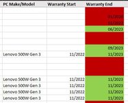
I have started playing with some conditional formatting and can get the sheets to highlight devices that are still in warranty and those that have expired but nothing in between. The sheet uses column G for warranty expiration date (in MM/YYYY format) and I have 3 rules setup currently: -

Row 1 - Formula=TRUE (used as header/title row)
Column G - Cell Value > TODAY() (Formats cell fill to Green to highlight still in warranty)
Column G - Cell Value < TODAY() (Formats cell fill to Red to highlight warranty expired)

I am not very good with Excel (last properly used it 20+ years ago in college) and have learned this from posts on this forum but would also like a rule to format the cells in Yellow if devices are within 6 months of warranty expiration. If this is possible and anyone can help, it would be most appreciated. Currently using Excel 2021 if that helps. Thanks in advance

 

[awoohaw]

Here is an attempt:

Mr excel questions 39.xlsm
	A	B	C	D	E	F	G
1	PC Make/Model	Warranty Start	Warranty End	checking date:	2023-05-31
2					<6 mos to exp	<12 mos to exp	expired
3			2020-01-01		FALSE	FALSE	TRUE
4			2022-01-01		FALSE	FALSE	TRUE
5			2022-06-01		FALSE	FALSE	TRUE
6			2022-12-01		FALSE	FALSE	TRUE
7			2023-03-01		FALSE	FALSE	TRUE
8			2023-05-15		FALSE	FALSE	TRUE
9			2023-05-29		FALSE	FALSE	TRUE
10			2023-05-30		FALSE	FALSE	TRUE
11			2023-05-31		TRUE	FALSE	FALSE
12			2023-06-01		TRUE	FALSE	FALSE
13			2023-09-01		TRUE	FALSE	FALSE
14			2023-11-28		TRUE	FALSE	FALSE
15			2023-11-29		TRUE	FALSE	FALSE
16			2023-11-30		TRUE	FALSE	FALSE
17			2023-12-01		FALSE	TRUE	FALSE
18			2023-12-02		FALSE	TRUE	FALSE
19			2023-12-03		FALSE	TRUE	FALSE
20			2023-12-04		FALSE	TRUE	FALSE
21			2024-05-15		FALSE	TRUE	FALSE
22			2024-05-29		FALSE	TRUE	FALSE
23			2024-05-30		FALSE	TRUE	FALSE
24			2024-05-31		FALSE	TRUE	FALSE
25			2024-06-01		FALSE	FALSE	FALSE
26			2024-06-02		FALSE	FALSE	FALSE
27			2024-06-01		FALSE	FALSE	FALSE
28	Lenovo 500W Gen 3	2022-11-01	2023-11-01		TRUE	FALSE	FALSE
29					FALSE	FALSE	TRUE
30	Lenovo 500W Gen 3		2023-11-01		TRUE	FALSE	FALSE
31	Lenovo 500W Gen 3		2023-11-01		TRUE	FALSE	FALSE
32	Lenovo 500W Gen 3		2023-11-01		TRUE	FALSE	FALSE
33	Lenovo 500W Gen 3		2023-11-01		TRUE	FALSE	FALSE
Bigdyl69

Cell Formulas
Range	Formula
E1	E1	=TODAY()
E3:E33	E3	=AND($E$1<=$C3,EDATE($E$1,6)>=C3)
F3:F33	F3	=AND(EDATE($E$1,6)<$C3,EDATE($E$1,12)>=$C3)
G3:G33	G3	=$C3<$E$1

Cells with Conditional Formatting
Cell	Condition		Cell Format	Stop If True
C3:C33	Expression	=$C3<$E$1	text	NO
C3:C33	Expression	=AND(EDATE($E$1,6)<$C3,EDATE($E$1,12)>=$C3)	text	NO
C3:C33	Expression	=AND($E$1<=$C3,EDATE($E$1,6)>=C3)	text	NO

 

[awoohaw]

In post 2 the rules are mutually exclusive so you do not have to indicate a "stop when true" as true can only happen once.
I learned to make conditional formatting formulas using the above to create formulas that will answer all of the scenarios I wish in columns (which is what I did with the three columns to the right). Then use the first formula in each column to set the conditional formatting rules, being sure that the relative/absolute cell referencing is maintained.

 

[Bigdyl69]

In post 2 the rules are mutually exclusive so you do not have to indicate a "stop when true" as true can only happen once.
I learned to make conditional formatting formulas using the above to create formulas that will answer all of the scenarios I wish in columns (which is what I did with the three columns to the right). Then use the first formula in each column to set the conditional formatting rules, being sure that the relative/absolute cell referencing is maintained.

Hi and thanks for the quick response. That has worked a treat (with a little cell reference manipulation) and does exactly what I want. I did swap the Green and Yellow highlighting around so Yellow highlights devices expiring within 6 months and Green is within 12 months. I assume that if the cell remains uncoloured that means the devices have in excess of 12 months warranty left? It seemed to indicate that in my testing anyway but it works great.

I'm going to use it as a template for all my schools and will share it with the other technicians (there are 5 of us working for the county/local authority) as it will make life so much easier for us and the schools for managing their IT assets.

Thank you so much for your help @awoohaw

 

[awoohaw]

Sorry I had the colors reversed. I was more focused on the rules and not necessarily the colors, although I do strive for that accuracy as well.
I'm happy you found a solution here.

regarding the unformatted cells, I only gave formulas for the three conditions i thought you requested. So what ever condition doesn't fit in those 3 scenarios will be unformatted.

Best wishes!