Formatting VBA Needed

[nrguerrieri]

Hello,

So i have an excel table with 9 columns and 10,000 rows. I would like every row in column C to be searched and every cell checks the other cells in column C for any other cell with the same 5 starting characters and then each one that is the same as the other. Those cells have their entire row filled in light grey.

Thanks,

Nick

 

[smozgur]

I am not sure about the performance, but is it ok to use Conditional Formatting in your project?

I selected A1 cell in the worksheet then I clicked on Conditional Formatting->Manage Rules->New Rule, and selected the "Use a formula to determine which cells to format" option. Selected Format, and set the Fill with gray.
Then I entered the following formula in the "Format values where this formula is true" text box. This is basically checking if cell is not blank and has another cell starting with the same first 5 chars.

=AND(NOT(ISBLANK($C1)), COUNTIF($C:$C,LEFT($C1,5) & "*")>1)

Clicked OK, and the new rule is in the list. I changed the "Applies to" field to be "$A:$I", and clicked OK.
(In fact, if the row count is certainly limited then may be you might want to use $A1:$I10000 instead of entire column, and use $C1:$C10000 in the formula above if it makes any difference for the performance. I actually tested it with 10K rows in 9 columns, and I didn't notice any problem.)

And I got all the rows with this criteria is gray.

Is this something that will help you?

Note: I am a VBA person, but if any non-VBA method is possible, then I prefer to go with it as long as it is not bad for the performance. Honestly, the VBA method might be even more performance killer for this question.

 

[nrguerrieri]

I am not sure about the performance, but is it ok to use Conditional Formatting in your project?

I selected A1 cell in the worksheet then I clicked on Conditional Formatting->Manage Rules->New Rule, and selected the "Use a formula to determine which cells to format" option. Selected Format, and set the Fill with gray.
Then I entered the following formula in the "Format values where this formula is true" text box. This is basically checking if cell is not blank and has another cell starting with the same first 5 chars.

=AND(NOT(ISBLANK($C1)), COUNTIF($C:$C,LEFT($C1,5) & "*")>1)

View attachment 26407

Clicked OK, and the new rule is in the list. I changed the "Applies to" field to be "$A:$I", and clicked OK.
(In fact, if the row count is certainly limited then may be you might want to use $A1:$I10000 instead of entire column, and use $C1:$C10000 in the formula above if it makes any difference for the performance. I actually tested it with 10K rows in 9 columns, and I didn't notice any problem.)

View attachment 26409

And I got all the rows with this criteria is gray.

Is this something that will help you?

Note: I am a VBA person, but if any non-VBA method is possible, then I prefer to go with it as long as it is not bad for the performance. Honestly, the VBA method might be even more performance killer for this question.

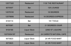
Hey thanks for the response. Doesnt seem to be working. See image. Looks like some things are being grayed out when their is no duplicate like 125 lounge and some arent greyed out when their is a suplicate like the 24 hour food mart.

 

[smozgur]

Are you sure that you selected A1 before creating the conditional formatting? It is the most important step.

 

[nrguerrieri]

Are you sure that you selected A1 before creating the conditional formatting? It is the most important step.

That was it! It is now fixed. Thank you sir!

I also have another question. Not sir if its worth doing a new post but I am trying to make a drop down list of that column c but in alphabetical order. Then when that name gets selected. It finds it in the list and strikethroughs the row with that business name.

 

[smozgur]

That was it! It is now fixed. Thank you sir!

You're welcome. Glad to hear it helps.

Regarding the other question, I believe you can still use the Conditional Formatting.
However, I am not sure how you need it.
Are you going to create the drop down separately, or do you need the dropdown to be filled by using the unique values in the column C?
Where are you going to put the dropdown? Somewhere on the worksheet?
Only one business name row will be strikethrough?

If you could answer these questions, then I'll try to help with that part as well since I think it could be still solved by using the same method.

Note: You can create a new question or you can continue here but then you might want to unmark the answer you selected above, so other helpers won't think that this question has been already answered. Just in case if someone else can help faster than I can. However, please just make sure to marking a solution again once you receive an answer which solves your question. In fact, you might even consider revisiting your old questions to mark a solution for the ones you have an answer. Here is the link that you can use to access your question list: Your unsolved questions

 

[smozgur]

@nrguerrieri : I closed the new question that you posted since you decided to unmark the solution in this question, and this thread also has more details about your question.
Please do not create new threads for the same questions - Rule 12 for more details.

 

[smozgur]

Additional question: What is your Office version? (You can set this information in your account to let helpers to know your Office version and platform, so they can provide compatible solutions).

For Office 365, we can use UNIQUE and SORT functions (available in 365) to create a data validation list. Here how I set it up in my worksheet for the same data structure in the original question.

I wrote the following formula in cell K1.

=SORT(UNIQUE(OFFSET($C$1,1,,COUNTA($C:$C)-1,1)))

This creates a unique list of business names in the column C as shown below. Since UNIQUE and SORT are spilling functions, the list goes down as much as necessary.

Then I selected cell L1, and created a List data validation with the following formula:

=$K$1#

So, this is the result:

You can preferably hide the column K.

Now, the Conditional Formatting step.
I selected A1 cell in the worksheet again, then I clicked on Conditional Formatting->Manage Rules->New Rule, and selected the "Use a formula to determine which cells to format" option. Selected Format, and set the Font as Strikethrough.
Then I entered the following formula in the "Format values where this formula is true" text box. This is basically checking if cell is not blank, and matches the current cell value with the currently selected business name in cell L1. This is also matching the first 5 chars as I assume you still need this here as well. If full match is required, then the formula could be updated by removing the LEFT function.

=AND(NOT(ISBLANK($C1)), LEFT($C1,5) = LEFT($L$1,5))

Clicked OK, and the new rule is in the list with the previous rule I created. I changed the "Applies to" field to be "$A:$I", and clicked OK.

And I got all the rows matching with the selected business name (first 5 chars) in cell L1 as strikethrough as show below, previous conditional formatting rule is also applied:

Hope this helps.

 

[nrguerrieri]

Additional question: What is your Office version? (You can set this information in your account to let helpers to know your Office version and platform, so they can provide compatible solutions).

For Office 365, we can use UNIQUE and SORT functions (available in 365) to create a data validation list. Here how I set it up in my worksheet for the same data structure in the original question.

I wrote the following formula in cell K1.

=SORT(UNIQUE(OFFSET($C$1,1,,COUNTA($C:$C)-1,1)))

This creates a unique list of business names in the column C as shown below. Since UNIQUE and SORT are spilling functions, the list goes down as much as necessary.
View attachment 26456

Then I selected cell L1, and created a List data validation with the following formula:

=$K$1#

View attachment 26457

So, this is the result:
View attachment 26458
You can preferably hide the column K.

Now, the Conditional Formatting step.
I selected A1 cell in the worksheet again, then I clicked on Conditional Formatting->Manage Rules->New Rule, and selected the "Use a formula to determine which cells to format" option. Selected Format, and set the Font as Strikethrough.
Then I entered the following formula in the "Format values where this formula is true" text box. This is basically checking if cell is not blank, and matches the current cell value with the currently selected business name in cell L1. This is also matching the first 5 chars as I assume you still need this here as well. If full match is required, then the formula could be updated by removing the LEFT function.

=AND(NOT(ISBLANK($C1)), LEFT($C1,5) = LEFT($L$1,5))

Clicked OK, and the new rule is in the list with the previous rule I created. I changed the "Applies to" field to be "$A:$I", and clicked OK.

View attachment 26461

And I got all the rows matching with the selected business name (first 5 chars) in cell L1 as strikethrough as show below, previous conditional formatting rule is also applied:

View attachment 26462

Hope this helps.

Thank you so much for your time.

I just updated my office version on my profile. It is 365.

Also the list you created using the unique function. It is pulling every row which I only want it to show only the visible business names as this is a table where I can filtering certain things.

I think if we fix that. This should work. Also, is there a way to do this without having to creating another column list? Just wondering, worst case I can just hide the cells or column that has this second created list.

Thanks,

 

[nrguerrieri]

Also, I would like to mak

Thank you so much for your time.

I just updated my office version on my profile. It is 365.

Also the list you created using the unique function. It is pulling every row which I only want it to show only the visible business names as this is a table where I can filtering certain things.

I think if we fix that. This should work. Also, is there a way to do this without having to creating another column list? Just wondering, worst case I can just hide the cells or column that has this second created list.

Thanks,

Additional question: What is your Office version? (You can set this information in your account to let helpers to know your Office version and platform, so they can provide compatible solutions).

For Office 365, we can use UNIQUE and SORT functions (available in 365) to create a data validation list. Here how I set it up in my worksheet for the same data structure in the original question.

I wrote the following formula in cell K1.

=SORT(UNIQUE(OFFSET($C$1,1,,COUNTA($C:$C)-1,1)))

This creates a unique list of business names in the column C as shown below. Since UNIQUE and SORT are spilling functions, the list goes down as much as necessary.
View attachment 26456

Then I selected cell L1, and created a List data validation with the following formula:

=$K$1#

View attachment 26457

So, this is the result:
View attachment 26458
You can preferably hide the column K.

Now, the Conditional Formatting step.
I selected A1 cell in the worksheet again, then I clicked on Conditional Formatting->Manage Rules->New Rule, and selected the "Use a formula to determine which cells to format" option. Selected Format, and set the Font as Strikethrough.
Then I entered the following formula in the "Format values where this formula is true" text box. This is basically checking if cell is not blank, and matches the current cell value with the currently selected business name in cell L1. This is also matching the first 5 chars as I assume you still need this here as well. If full match is required, then the formula could be updated by removing the LEFT function.

=AND(NOT(ISBLANK($C1)), LEFT($C1,5) = LEFT($L$1,5))

Clicked OK, and the new rule is in the list with the previous rule I created. I changed the "Applies to" field to be "$A:$I", and clicked OK.

View attachment 26461

And I got all the rows matching with the selected business name (first 5 chars) in cell L1 as strikethrough as show below, previous conditional formatting rule is also applied:

View attachment 26462

Hope this helps.

Also, instead of a strikethrough. Can we make it so the whole row turns into a green fill?

Then I would like to make a last column that says "On-Boarded'". Then for each row that has green fill, the last column will say "Yes". To show we got that business.