Formula for automating the ordering of a table

[mteden]

Hi there,

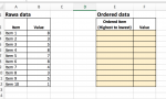
I want to set up a spreadsheet where I will be updating several input tables with raw data. I then want that raw data to be automatically transferred to a separate table, where it will need to be ordered to present from the highest value at the top to the lowest value at the bottom. The raw data table will not be ordered in this way (it will probably be ordered in sequence of the items (e.g. Item 1, Item 2 etc).

Is there a way that I can have a formula that automatically copies the values over AND orders them in the correct order (e.g. from highest to lowest)? If so, how do I do this?

Below is an image of some example tables that I might use. Although my actual tables will be much larger. I am not sure if it is possible to attach the actual spreadsheet here, is it?

Thanks
J

 

[Toadstool]

Hi MTeden,

Does this do what you want?

MTeden.xlsx
	A	B	C	D	E	F
1	Raw Data				Ordered Data
2	Item	Value			Item	Value
3	Item 1	8			Item 1	8
4	Item 2	3			Item 4	8
5	Item 3	5			Item 6	8
6	Item 4	8			Item 5	7
7	Item 5	7			Item 3	5
8	Item 6	8			Item 9	5
9	Item 7	4			Item 7	4
10	Item 8	3			Item 2	3
11	Item 9	5			Item 8	3
12	Item 10	2			Item 10	2
Sheet1

Cell Formulas
Range	Formula
E3:E12	E3	=IFERROR(INDEX($A$3:$A$999,AGGREGATE(15,6,ROW($A$3:$A$999)-ROW($A$2)/($B$3:$B$999=F3),COUNTIF($F$3:F3,F3))),"")
F3:F12	F3	=AGGREGATE(14,6,$B$3:$B$999,ROW()-ROW($F$2))

 

[mteden]

It does yes! Thanks for that. Although I have no idea how to follow the formula.

Will this simply be able to be copied down larger ranges, and adjust the source columns?

Many thanks!

 

[Toadstool]

You'd need to adjust the $999 parts of the formula if you use more rows than that. The starting row and columns match your screenshot.

I should have added an error check on column F so let me give you a revised version then explain how it works:

MTeden.xlsx
	A	B	C	D	E	F
1	Raw Data				Ordered Data
2	Item	Value			Item	Value
3	Item 1	8			Item 1	8
4	Item 2	3			Item 4	8
5	Item 3	5			Item 6	8
6	Item 4	8			Item 5	7
7	Item 5	7			Item 3	5
8	Item 6	8			Item 9	5
9	Item 7	4			Item 7	4
10	Item 8	3			Item 2	3
11	Item 9	5			Item 8	3
12	Item 10	2			Item 10	2
Sheet1

Cell Formulas
Range	Formula
E3:E12	E3	=IF(F3="","",(INDEX($A$3:$A$999,AGGREGATE(15,6,ROW($A$3:$A$999)-ROW($A$2)/($B$3:$B$999=F3),COUNTIF($F$3:F3,F3)))))
F3:F12	F3	=IFERROR(AGGREGATE(14,6,$B$3:$B$999,ROW()-ROW($F$2)),"")

So the formula in column F obviously need to be copied down as far as your Raw data rows.

=IFERROR(AGGREGATE(14,6,$B$3:$B$999,ROW()-ROW($F$2)),"")

The IFERROR traps the error when you run out of raw data rows and puts in a null.
The AGGREGATE option 14 says get the value from the specified rows B3 to B999 which is the ROW()-ROW($F$2) highest. The first entry will return row 3 minus row 2 so a one and gets the 1st highest number, an eight.
The next entry in row four gets the row 4 minus row 2 so 2nd highest entry, which is also an eight, etc.

Column E formula also needs to be copied down as many rows as you have raw data.

=IF(F3="","",(INDEX($A$3:$A$999,AGGREGATE(15,6,ROW($A$3:$A$999)-ROW($A$2)/($B$3:$B$999=F3),COUNTIF($F$3:F3,F3)))))

The IF says if there's no Value found in column F then return a null.
The INDEX($A$3:$A$999 says return the text from column A for the row returned by the AGGREGATE.
AGGREGATE(15,6,ROW($A$3:$A$999)-ROW($A$2) says get the nth lowest row number from A3 to A999 but minus Row 2 so the returned number will start at one.
/($B$3:$B$999=F3) says divide each row by the result of a check if the B3 to B999 equals F3, so at first it's looking for the highest value, an eight. If it finds an eight then it's a logical 1, so the row divided by the 1 returns the row. If it's not an eight it returns 0 which causes the row number between b3 and b999 to be divided by zero and the zerodivide is trapped by the AGGREGATE 6 option and ignored.
The COUNTIF($F$3:F3,F3) tells aggregate which nth lowest value to find, so for row 3 it find one 8 and returns 1 so it returns the lowest row number with an 8 whichIndex uses to get the "Item 1" text. On row 4 it finds there's two 8s so it looks for the row with the second highest number, another 8 in row 6 so you get "Item 4", etc.

 

[mteden]

This is brilliant. Thank you.

 

[Toadstool]

You're welcome!

 

[Peter_SSs]

I suggest that you update your Account details (click your user name at the top right of the forum) so helpers always know what Excel version(s) & platform(s) you are using as the best solution often varies by version. For example, IF you have Excel 365 and it includes the SORTBY function here is a very easy way.

1. If it isn't already, turn the raw data table (A2:B12 in your image) into a formal Excel table by selecting that range then on the Insert ribbon tab -> Table -> My Table has headers -> OK

2. Then in cell E3 only put the formula shown below. The other results will automatically 'spill' down and across. Further, if you add more rows to the 'raw' table the results will automatically update (including adding or reducing rows) without anything further being done.

20 03 15.xlsm
	A	B	C	D	E	F
1	Raw Data				Ordered Data
2	Item	Value			Item	Value
3	Item 1	8			Item 1	8
4	Item 2	3			Item 4	8
5	Item 3	5			Item 6	8
6	Item 4	8			Item 5	7
7	Item 5	7			Item 3	5
8	Item 6	8			Item 9	5
9	Item 7	4			Item 7	4
10	Item 8	3			Item 2	3
11	Item 9	5			Item 8	3
12	Item 10	2			Item 10	2
13
Order Table

Cell Formulas
Range	Formula
E3:F12	E3	=SORTBY(Table1,Table1[Value],-1)
Dynamic array formulas.

 

[mteden]

Thanks @Peter_SSs.

I have updated my profile. As it turns out I do have 365 and the SortBy function. I run on a MacOS platform. I've added that to my profile so that this is easily available. Many thanks.

Thanks again also, @Toadstool! You've both helped immensely.

 

[Peter_SSs]

I have updated my profile.

Thanks for that.

As it turns out I do have 365 and the SortBy function.

Good news! The new dynamic array formulas are very powerful, making tasks like this so much simpler than they used to be.