Formula Query

[dcwinter]

Hello All,

This is quite complicated so please bear with me.

I have a list of data with staff names (in column E) and then Minutes (column F). So the data looks like this:

STAFF MEMBER MINUTES
Staff B -599
Staff C -599
Staff D 60
Staff A 60
Staff B 60
Staff C -39

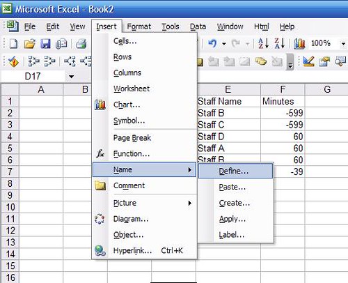
On another sheet I have a table like this:

STAFF MEMBER Poor Fair Good Excellent
Staff A
Staff B
Staff C
Staff D


What I want to be able to do is add up the number of times a staff member falls between 0 and above (Excellent); -0.1 and -15 for Good; -15.1 and -30 for Fair and then -30 and below for Poor.

Based on the above example, Staff be would have 1 against Poor and 1 against Excellent.

I hope this makes sense. I don't know where to start!!!

Many Thanks

DC

 

[gardnertoo]

Assuming your data is on Sheet1 and the results on Sheet2:

On Sheet1 I created two named ranges. Staff_Name refers to:

=OFFSET(Sheet1!$E$1,1,0,COUNTA(Sheet1!$E:$E)-1,1)

"Minutes" refers to:

=OFFSET(Sheet1!$F$1,1,0,COUNT(Sheet1!$F:$F),1)

Then on Sheet2, I build this:

Book2
	A	B	C	D	E
1	Criteria:	-30	-15	0	1000000
2	Staff Member	Poor	Fair	Good	Excellent
3	Staff A	0	0	0	1
4	Staff B	1	0	0	1
5	Staff C	2	0	0	0
6	Staff D	0	0	0	1
Sheet2

The formula in column B is unique. From column C over, you can enter the column C formula and copy it to the right.

 

[PATSYS]

Assuming the sheet that contains the data is called Sheet1 and the table on the other sheet, the cell for staff member A and Poor is on cell B2.

On cell B2, paste this formula:

=SUMPRODUCT((Sheet1!$A$2:$A$7=$A2)*((B$1="Poor")*(Sheet1!$B$2:$B$7<-30)))+SUMPRODUCT((Sheet1!$A$2:$A$7=$A2)*((B$1="Fair")*(Sheet1!$B$2:$B$7>=-30)*(Sheet1!$B$2:$B$7<-15.1)))+SUMPRODUCT((Sheet1!$A$2:$A$7=$A2)*((B$1="Good")*(Sheet1!$B$2:$B$7>=-15)*(Sheet1!$B$2:$B$7<-0.1)))+SUMPRODUCT((Sheet1!$A$2:$A$7=$A2)*((B$1="Excellent")*(Sheet1!$B$2:$B$7>=0)))

copy to all the rest of the cells in the table.

 

[jasonb75]

I think Gardnertoo's idea is better, but I'll post this anyway, this was done in 1 sheet but could work with 2 just as easily.

Excel Workbook
	A	B	C	D	E
1	STAFF MEMBER	MINUTES
2	Staff B	-599
3	Staff C	-599
4	Staff D	-22
5	Staff A	60
6	Staff B	60
7	Staff C	-39
8
9
10
11
12	STAFF MEMBER	Poor	Fair	Good	Excellent
13	Staff A	0	0	0	1
14	Staff B	1	0	0	1
15	Staff C	2	0	0	0
16	Staff D	0	1	0	0
Sheet2

 

[dcwinter]

hI,

Thanks for the quick reply!

I'm just slightly confused about your reply - I don't actually know what a named range is...

Also, to explain where the data is properly:

The 'Poor, Good, Fair, Excellent' Table is on a sheet named 'Tables' and starts in cell D31.

The data it is looking at is on a sheet called 'Report' and is in columns E and F.

I'm not very good am I?!!

Many Thanks

DC

****** I'LL TRY JASONB75'S APPROACH BECAUSE IT LOOKS LIKE I CAN BREAK IT UP A LITTLE EASIER SO THANKS VERY VERY MUCH!!! ********

 

[PATSYS]

When you said

"The 'Poor, Good, Fair, Excellent' Table is on a sheet named 'Tables' and starts in cell D31."

I assume the the intersection of Staff A and Poor is in cell E32 then?

If so, paste this in cell E32 and copy to the rest of the table:

=SUMPRODUCT((Report!$E$2:$E$7=$D32)*((E$31="Poor")*(Report!$F$2:$F$7<-30)))+SUMPRODUCT((Report!$E$2:$E$7=$D32)*((E$31="Fair")*(Report!$F$2:$F$7>=-30)*(Report!$F$2:$F$7<-15.1)))+SUMPRODUCT((Report!$E$2:$E$7=$D32)*((E$31="Good")*(Report!$F$2:$F$7>=-15)*(Report!$F$2:$F$7<-0.1)))+SUMPRODUCT((Report!$E$2:$E$7=$D32)*((E$31="Excellent")*(Report!$F$2:$F$7>=0)))

Note: It would really be easier if you paste your actual table, that way we can be specific as to which cell you should paste the formula and copy to which range.

 

[Dave Patton]

Staff Member
Insert a row and include threshold numbers (example uses row13) see Jason's example
							
	Poor	Fair	Good	Excellent			
	-30.01	-30	-15	0			
A	0	0	0	1			
B	1	0	0	1			
C	2	0	0	0			
D	0	0	0	1				


With correct numbers in B13:E13								
B14 =SUMPRODUCT(--($A$2:$A$9=A14),--($B$2:$B$9 <   B$13))							
C14 =SUMPRODUCT(--($A$2:$A$9=$A14),--($B$2:$B$9 >  C$13),--($B$2:$B$9 <  D$13))							
D14 =SUMPRODUCT(--($A$2:$A$9=$A14),--($B$2:$B$9 > =D$13),--($B$2:$B$9 < E$13))							
E14 =SUMPRODUCT(--($A$2:$A$9=$A14),--($B$2:$B$9 > =E$13))

N.B. You do not have array enter SumProduct formulas.

 

[gardnertoo]

I'm not very good am I?!!

Everybody here started out where you are, so don't worry. Besides, based on your signature, you seem to have the right attitude!

Named ranges: This is a very useful tool which allows you to replace references like $A$2:$A$102 with a plain-language name like "staff_names". From my experience, this has two practical advantages. One, I can more easily remember that my staff names are located at the named range "staff_names", and less easily remember that they are located in the range of E2:E20 or whatever. Two, named ranges can be set up with dynamic formulas (as I have done here) which makes Excel keep track of how much data there is. If we specify that the formula should look to E2:E20, when you get a score in row 21 it will be ignored until you go back and change all the formulas to cover the new rows. Using the named range with dynamic formulas to determine the extent of the data frees us from having to keep track of it manually.

I use named ranges a lot, especially if the data range is subject to changes going forward. In your case, it looks like you will be adding rows in the future, as various staff members get new time scores.

To create a name, click on "Insert", then "Name", then "Define.."

This is how you tell excel what cells you want to include in the named range. It can be as simple as referring to a fixed range of cells, like $A$1:A$A12, or a formula like I've done here:

 

[Dave Patton]

I agree with Gardnertoo about Named Ranges.

If you use Excel 2003, look at Data List; Excel 2007 has a similiar feature.

With Data List, the formula will expand with new entries. This works whether you name the ranges or not. You do not have to define the ranges as Dynamic named ranges.

 

[dcwinter]

You guys are all fantastic!!!!!

Cheers!