Formula question

[Cr4ig]

Morning you smart people, i have tried a few different ways , but struggling, it look like my last post asking this question was removed for some reason? can anyone tell me what the formula would be for this please?

 

[etaf]

not following
formula to do what - you dont show any examples of results

from the Table
code H with a Score of 9 - shows a grade of 5 , not 4 as highlighted -
also why is F , 5 highlighted ?

are you using version 2016
if later version MAXIFS()

or a 2 criteria lookup
but just need to know what you want exactly

Excel MAX IF formula to find largest value with conditions

MAX IF formula examples to get the max value in Excel based on one or several conditions that you specify.

www.ablebits.com

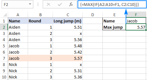
{=MAX(IF(criteria_range1=criteria1, IF(criteria_range2=criteria2, max_range)))}
{=MAX(IF((criteria_range1=criteria1) * (criteria_range2=criteria2), max_range))}

Note: Images are difficult to see , and also requires that I input all the data myself, which means I may make an error, which is very time consuming, and from my point of view less likely to get a response, if a complicated spreadsheet. Plus we cannot see any of the formulas used.

Therefore -

A SMALL sample spreadsheet, around 10-20 rows, would help a lot here, with all sensitive data removed, and expected results mocked up and manually entered, with a few notes of explanation.

MrExcel has a tool called “XL2BB” that lets you post samples of your data and will allow us to copy/paste your sample data into our Excel spreadsheets, saving a lot of time.

XL2BB - Excel Range to BBCode

Excel 'mini-sheet' in messages - XL2BB Although experts prefer to read your description and question instead of working in your actual file to solve your problem, there are times that it is difficult to explain an issue without providing actual...

www.mrexcel.com

You can also test to see if it works ok, in the "Test Here" forum.

Test Here

Use this forum to test your signature, learn bbcode, smilies, XL2BB, etc. Threads in this forum are automatically deleted after no replies for seven (7) days

www.mrexcel.com

OR if you cannot get XL2BB to work, or have restrictions on your PC , then put the sample spreadsheet onto a share
I only tend to goto OneDrive, Dropbox or google docs , as I'm never certain of other random share sites and possible virus.
Please make sure you have a representative data sample and also that the data has been desensitised, remember this site is open to anyone with internet access to see - so any sensitive / personal data should be removed

 

[Cr4ig]

Sorry if this is not making sense, Result should be in Cell G7, its looking at E7 & F7, Range A & B with the result from C, the orange numbers are probably confussing things ignore them i should have taken them out before posting sorry.

CC

 

[hrayani]

Hello,

try

Book6
	A	B	C	D	E	F	G
1
2	Code	Score	Grade
3	H	1	4
4	H	2	4
5	H	3	4				Result
6	H	4	4		Code	Score	Grade
7	H	5	4		H	9	5
8	H	6	4
9	H	7	4
10	H	8	5
11	H	9	5
12	F	10	4
13	F	11	4
14	F	12	4
15	F	13	4
16	F	14	4
17	F	15	5
18	F	16	5
19	F	17	5
20	F	18	5
Sheet1

Cell Formulas
Range	Formula
G7	G7	=INDEX(C3:C20,MATCH(1,(E7=A3:A20)*(F7=B3:B20)),0)
Press CTRL+SHIFT+ENTER to enter array formulas.

 

[Cr4ig]

Thank You

 

[etaf]

you have an answer now - also posted with an answer here

Formula required please

Morning, I am not sure if i was doing it right but could someone tell me what formula you would use for the below please? Code Score Grade H 1 4 H 2 4 H 3 4 Result H 4 4 Column D Column Z Column AB H 5 4 Code Score Grade H 6 4 H 9 Formula H 7 4...

www.mrexcel.com

using the MAX(IF as suggested

Book3
	A	B	C	D	E	F	G	H	I
1
2	Code	Score	Grade
3	H	1	4
4	H	2	4
5	H	3	4				Result
6	H	4	4		Code	Score	Grade		Maxif
7	H	5	4		H	9	5		5
8	H	6	4
9	H	7	4
10	H	8	5
11	H	9	5
12	F	10	4
13	F	11	4
14	F	12	4
15	F	13	4
16	F	14	4
17	F	15	5
18	F	16	5
19	F	17	5
20	F	18	5
21
Sheet1

Cell Formulas
Range	Formula
G7	G7	=INDEX(C3:C20,MATCH(1,(E7=A3:A20)*(F7=B3:B20)),0)
I7	I7	=MAX(IF((A3:A20=E7) * (B3:B20=F7),C3:C20))

 

[sparky2205]

=XLOOKUP(E7&F7,Code&Score,Grade)

Where Code = A3:A20 and Score = B3:B20 and Grade = C3:C20

I would use named ranges as above and also create each column as a table.
The advantage of this being if you add data to your spreadsheet it will automatically be incorporated into the formula.