SirGruffles
New Member
- Joined
- Jul 23, 2018
- Messages
- 26
Apologies if this looks/sounds messy...
In the middle of my (probably unnecessarily complex/large) formula, I have this function: (OFFSET(INDIRECT(ADDRESS(ROW(), COLUMN())),-ROW()+2,0))
As it stands, this will pull the value of the cell 2 rows from the top, in the same column as the current cell.
While this works great for the first "area" of data (January 2020 in this instance), if I copy it down into the sections for other months, it will continue to pull January data only.
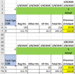
I attached a fragment of the worksheet to this post for some visual assistance.
The type of formula I'm looking for, in words I can only hope I'm using correctly:
1) Would function similarly to what's currently there, but
2) Would allow for pasting down into other months
a) In the picture, the 39 & 134 are correct in the January area, but are incorrect for the February area, as February has not occurred yet. It is still pulling that 1/4/2020 date value from the 2nd row.
b) Using a different variation of OFFSET... allowed me to easily code the "future" months, but gave me issues when pasting down the line of the current month. As going from Row 6 to Row 7 would take the OFFSET cell's value a cell down.
Is there a different way to use OFFSET and ADDRESS that would allow me to "lock" that specific month row (rows 2 & 69 in the picture) in their respective months? (Instead of my -ROW()+2 formula).
If more of the formula is needed for clarity, let me know and I can post more.
The goal here is to create a formula I can use in each month's sections, and not having to create a different one for each month OR for each line (A,B,etc).
I appreciate any advice, tips, ideas.
Thank you for your time.
In the middle of my (probably unnecessarily complex/large) formula, I have this function: (OFFSET(INDIRECT(ADDRESS(ROW(), COLUMN())),-ROW()+2,0))
As it stands, this will pull the value of the cell 2 rows from the top, in the same column as the current cell.
While this works great for the first "area" of data (January 2020 in this instance), if I copy it down into the sections for other months, it will continue to pull January data only.
I attached a fragment of the worksheet to this post for some visual assistance.
The type of formula I'm looking for, in words I can only hope I'm using correctly:
1) Would function similarly to what's currently there, but
2) Would allow for pasting down into other months
a) In the picture, the 39 & 134 are correct in the January area, but are incorrect for the February area, as February has not occurred yet. It is still pulling that 1/4/2020 date value from the 2nd row.
b) Using a different variation of OFFSET... allowed me to easily code the "future" months, but gave me issues when pasting down the line of the current month. As going from Row 6 to Row 7 would take the OFFSET cell's value a cell down.
Is there a different way to use OFFSET and ADDRESS that would allow me to "lock" that specific month row (rows 2 & 69 in the picture) in their respective months? (Instead of my -ROW()+2 formula).
If more of the formula is needed for clarity, let me know and I can post more.
The goal here is to create a formula I can use in each month's sections, and not having to create a different one for each month OR for each line (A,B,etc).
I appreciate any advice, tips, ideas.
Thank you for your time.
")


