Formula to calculate values in current row and above only

[germany1403]

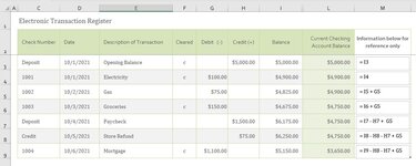
Hello, everyone! I am trying to modify an electronic transaction register (see attached image), so that it will make it easier for me to balance my transactions with my actual checking account balance in my bank. Everything is working great with the exception of column L. Column L is supposed to auto-calculate the account balance based on transactions that have not yet cleared (empty cells in column F).

Example: Cell I8 reflects $6,250.00. L8 is supposed to take that value plus or minus all of the transactions that have not yet cleared. In this case, L8 should auto generate the following formula: I8 - H8 - H7 + G5. Calculations should only include current row values and above.

For reference, I added a faux column "M" that outlines what the formula is supposed to reflect for each field in column L.

I know this is a complicated question, but am hoping that someone can follow my train of thought. Please let me know if you have any questions and thanks in advance for all forthcoming responses.

 

[Anthony47]

Ignoring your approach, I seem that you might use in L3:

=SUM(H$3:H3)-SUM(G$3:G3)

Then copy down

Bye

 

[Fluff]

How about in L3 dragged down

=SUMIFS(H$3:H3,F$3:F3,"c")-SUMIFS(G$3:G3,F$3:F3,"c")

 

[germany1403]

Ignoring your approach, I seem that you might use in L3:

=SUM(H$3:H3)-SUM(G$3:G3)

Then copy down

Bye

Hello Anthony47, thank you very much for your reply. I tried it, but it did not accomplish the task. The formula that Fluff posted actually did the trick. Thanks for responding though- I appreciate it.

 

[germany1403]

How about in L3 dragged down

=SUMIFS(H$3:H3,F$3:F3,"c")-SUMIFS(G$3:G3,F$3:F3,"c")

THANK YOU, THANK YOU, THANK YOU! Your formula worked and accomplished exactly what I hoped it would do. Thanks again for taking the time to respond. Much appreciate it!

 

[Fluff]

Glad we could help & thanks for the feedback.