Formula to copy a cell (word) if another cell is 0 and create a list from the words

[jbillyo]

I have a spreadsheet with xlookup to generate a total using a dropdown menu for a spelling test.
On the sheet, I have a list of 103 words and I have used 1 for right, 0 for wrong.
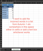
What I now want to do is use the value 0 (wrong answer) to generate a list of words when a name is selected from the dropdown menu.
I assume this is possible but it is beyond me.

Thanks in advance,
John

 

[Eric W]

It depends on how your sheet is set up, but something like this maybe:

Book1
	A	B	C	D	E	F	G	H
1	Name		Word		Ann	Bob	Cal	Diana
2	Cal		dog		1	1	1	0
3			cat		1	0	1	0
4	Misspelled words		pachyderm		1	1	0	1
5	pachyderm		orca		1	0	0	1
6	orca		mouse		1	1	1	0
7	capybara		capybara		1	0	0	1
8			moose		1	1	1	0
Sheet4

Cell Formulas
Range	Formula
A5:A7	A5	=FILTER(C2:C8,INDEX(E2:H8,0,MATCH(A2,E1:H1,0))=0)
Dynamic array formulas.

 

[jbillyo]

I hope this makes it a little clearer

 

[jbillyo]

Thank you for the quick reply Eric.
I have tried to substitute the formula with what I think is the same information but it comes up with an error.
Any ideas?

=FILTER('Autumn 1 2021'!B4:B106,INDEX('Autumn 1 2021'!'Autumn 1 2021'!'Autumn 1 2021'!:'Autumn 1 2021'!C4:R106,0,MATCH('Pupil Analysis'!A1:B1,'Autumn 1 2021'!C3:R3,0))=0)

 

[Eric W]

I tried to replicate your workbook based on the pictures, but it took a bit. In the future, consider using the XL2BB tool (see my signature or the menu in the reply box), to make it easier to copy and test with.

But if this is a reasonable reproduction of your Autumn 1 2021 sheet:

Book1
	A	B	C	D	E	F
1
2		Oak 21/22
3		Year 5/6 CEW Analysis Sheet	A	B	C	D
4	1	accommodate	1	0	1	1
5	2	accompany	1	0	0	1
6	3	according	1	0	1	1
7	4	achieve	0	0	0	1
8	5	aggressive	0	0	1	1
9	6	amateur	1	0	0	0
10	7	ancient	1	0	1	1
11	8	apparent	0	0	1	1
12	9	appreciate	0	0	1	1
13	10	attached	0	0	1	1
Autumn 1 2021

then you should be able to do something like this:

Book1
	A	B	C	D	E	F	G	H
1	C
2	Term	Score
3	Autumn 1 2021	7	accompany	achieve	amateur	0	0	0
4	Autumn 2
5	Spring 1
6	Spring 2
7	Summer 1
8	Summer 2
9
Pupil Analysis

Cell Formulas
Range	Formula
B3	B3	=SUM(INDEX(INDIRECT("'"&A3&"'!C3:R106"),0,MATCH($A$1,INDIRECT("'"&A3&"'!C3:R3"),0)))
C3:CT3	C3	=TRANSPOSE(FILTER(INDIRECT("'"&A3&"'!B4:B106"),INDEX(INDIRECT("'"&A3&"'!C4:R106"),0,MATCH($A$1,INDIRECT("'"&A3&"'!C3:R3"),0))=0))
Dynamic array formulas.

Note that I put the whole sheet name in A3, so that the formulas could use it. You can just drag down the formulas if all the Term names are the sheet names. Also, the 0's running off to the right should not be a problem if you use the formula on your whole sheet, not just the subset I created.

See if this works for you.

 

[jbillyo]

You absolute legend!! Thank you so much. I would never have got there without your help!

 

[Eric W]

Happy to help! ?

 

[jbillyo]

Hi Eric,
Sorry to ask something else but is there a way that I can take the list of incorrect words and create either a multiple cell block e.g. 21 x 5 array of cells (incase all 103 words are incorrect) or in a text box floating above the spreadsheet.
I could then print out on an A4 sheet rather than multiple pages.
Thanks in advance
John

 

[Eric W]

Possibly. I set it up the way I did so that if you have multiple sheets (Autumn 1, Autumn 2, Spring 1, Spring 2, etc.), you could show all the words for all the sheets. If you put them in a block, then you'd have to rearrange things. Maybe like this:

Book1
	A	B	C	D	E	F	G	H	I	J	K	L	M	N	O
1	C
2	Term	Score							Term	Score
3	Autumn 1 2021	7	accompany	achieve	amateur	0	0		Autumn 2 2021	1	salt	pepper	oregano	thyme	mace
4			0	0	0	0	0				cinnamon	garlic	onion	saffron	0
5			0	0	0	0	0				0	0	0	0	0
6			0	0	0	0	0				0	0	0	0	0
7			0	0	0	0	0				0	0	0	0	0
8			0	0	0	0	0				0	0	0	0	0
9			0	0	0	0	0				0	0	0	0	0
10			0	0	0	0	0				0	0	0	0	0
11			0	0	0	0	0				0	0	0	0	0
12			0	0	0	0	0				0	0	0	0	0
13			0	0	0	0	0				0	0	0	0	0
14			0	0	0	0	0				0	0	0	0	0
15			0	0	0	0	0				0	0	0	0	0
16			0	0	0	0	0				0	0	0	0	0
17			0	0	0	0	0				0	0	0	0	0
18			0	0	0	0	0				0	0	0	0	0
19			0	0	0	0	0				0	0	0	0	0
20			0	0	0	0	0				0	0	0	0	0
21			0	0	0	0	0				0	0	0	0	0
22			0								0	0	0	0	0
23											0	0
24	Spring 1								Spring 2
25
26
27	Summer 1								Summer 2
Pupil Analysis

Cell Formulas
Range	Formula
B3,J3	B3	=SUM(INDEX(INDIRECT("'"&A3&"'!C3:R106"),0,MATCH($A$1,INDIRECT("'"&A3&"'!C3:R3"),0)))
C3:G23,K3:O23	C3	=IFERROR(INDEX(FILTER(INDIRECT("'"&A3&"'!B4:B106"),INDEX(INDIRECT("'"&A3&"'!C4:R106"),0,MATCH($A$1,INDIRECT("'"&A3&"'!C3:R3"),0))=0),SEQUENCE(21,5)),"")
Dynamic array formulas.

Again, you won't see the 0s on a full sheet, but you'll have to leave room for them. Or maybe just put a drop-down in A3 with the sheet names.

 

[jbillyo]

Thank you, will give it a go