Jyggalag

Active Member
Joined
Mar 8, 2021
Messages
422
Office Version
  1. 365
  2. 2019
Platform
  1. Windows
Hi all,

I currently have a data set that looks like this:

1662019084312.png


I would like to transpose my information down under columns H-L so that for ALL cells in A that contains "George", their respective cells in columns B-F will be transposed under column H.

Likewise the same for all cells that contain any of the titles in column I-L

The trick is that all the cells in column A contain the title in columns H-L, however I can't figure out how to get this done

I hope my question makes sense? Otherwise please let me know and I'll be happy to elaborate :)

@Fluff I think you may have done something similar to this before?

Kind regards,
Jygglaag
 

Excel Facts

Which lookup functions find a value equal or greater than the lookup value?
MATCH uses -1 to find larger value (lookup table must be sorted ZA). XLOOKUP uses 1 to find values greater and does not need to be sorted.
I can do something along these lines:

1662021422371.png


However, the issue for me is that:

1) I can only do if it cell itself is named "George", but I want it to be if the cell just contains the string "George" anywhere in its value at all

and

2) If I try to "pull" the formula down, it creates a spill:

1662021470877.png
 
Upvote 0
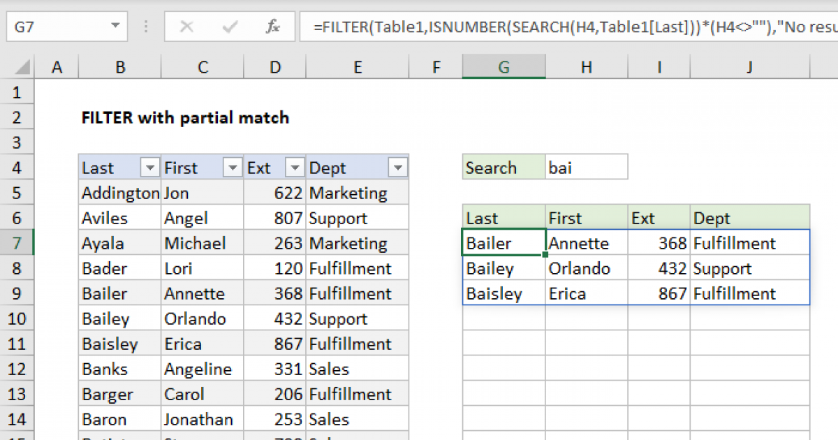
Two links I think may help with this:
Filter with Contains:
Flatten and stack output:
 
Upvote 0
Do you have the new functions such as TOCOL?
 
Upvote 0
If you do have TOCOL try
Excel Formula:
=TOCOL(FILTER($B$2:$F$22,ISNUMBER(SEARCH(H1,$A$2:$A$22))))
 
Upvote 0
Do you have the new functions such as TOCOL?
What is TOCOL and is it something I have to download externally, or is it automatically included in newer versions of Excel?

Also, apologies for the very late response!
 
Upvote 0
It's one of the new functions that has recently been released to the monthly channel & will probably be released to the semi-annual channel in January.
 
Upvote 0
Assuming you don't have TOCOL yet, another option is
Excel Formula:
=LET(f,FILTER($B$2:$F$22,ISNUMBER(SEARCH(H1,$A$2:$A$22))),c,COLUMNS(f),s,SEQUENCE(c*ROWS(f),,0),INDEX(f,INT(s/c)+1,MOD(s,c)+1))
 
Upvote 0

Forum statistics

Threads
1,214,864
Messages
6,121,981
Members
449,058
Latest member
oculus

We've detected that you are using an adblocker.

We have a great community of people providing Excel help here, but the hosting costs are enormous. You can help keep this site running by allowing ads on MrExcel.com.
Allow Ads at MrExcel

Which adblocker are you using?

Disable AdBlock

Follow these easy steps to disable AdBlock

1)Click on the icon in the browser’s toolbar.
2)Click on the icon in the browser’s toolbar.
2)Click on the "Pause on this site" option.
Go back

Disable AdBlock Plus

Follow these easy steps to disable AdBlock Plus

1)Click on the icon in the browser’s toolbar.
2)Click on the toggle to disable it for "mrexcel.com".
Go back

Disable uBlock Origin

Follow these easy steps to disable uBlock Origin

1)Click on the icon in the browser’s toolbar.
2)Click on the "Power" button.
3)Click on the "Refresh" button.
Go back

Disable uBlock

Follow these easy steps to disable uBlock

1)Click on the icon in the browser’s toolbar.
2)Click on the "Power" button.
3)Click on the "Refresh" button.
Go back
Back
Top