Larry of Oz
New Member
- Joined
- Jun 2, 2020
- Messages
- 17
- Office Version
- 2016
- Platform
- Windows
Hello gurus, I'm hoping someone can help with a solution that is escaping me no matter what I seem to try. I've found similiar problems on other threads, but not quite the right solution.
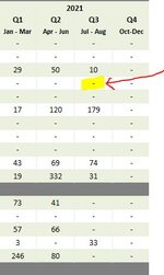
I have an Excel workbook to track the rollout of a project. On one worksheet are the locations of the project in rows, and the months in columns. If the project has NOT commenced, there is a dash (hyphen) in the column cell. for that month. If the project HAS commenced, a number referring to users is in the column cell for that month (note the number could be zero). A 'Locations' screenshot is attached.
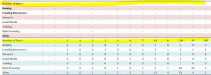
On my summary worksheet, to be used for reporting, I have been trying to come up with a formula that will pull in a total for the number of users by location per quarter OR enter a dash if each of the three quarter months shows a dash indicating the project hasn't commenced. I originally had the following formula:
=IF(SUM(Eastern!N5:P5)=0,"-",SUM(Eastern!N5:P5))
As luck would have it we have rolled out to a location that has had some issues, so though the project has commenced, the usage on the source document shows 0 (zero). Zero indicates project commenced but no usage. So in this case I need it to actually show a zero, not a dash. I tried something like the below but that didn't work either. It put dashes in three consecutive cells as the result.
=IFS(Western!V5:X5="-","-",Western!V5:X5>=0,"=SUM(Western!V5:X5)")
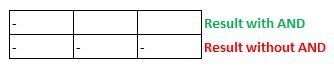
I feel like I've tried a million combinations of IF. IFS SUMIF, SUMIFS and just can't seem to find the right solution and my brain is become too scrambled to make headway. Also attaching a screenshot of an example using of output where I need the quarterly result to read 0 not ' (dash).
Thanks so very much for any advice you can offer. Kind regards, Lauren
O365 using Windows 10 and Excel desktop version 2102
I have an Excel workbook to track the rollout of a project. On one worksheet are the locations of the project in rows, and the months in columns. If the project has NOT commenced, there is a dash (hyphen) in the column cell. for that month. If the project HAS commenced, a number referring to users is in the column cell for that month (note the number could be zero). A 'Locations' screenshot is attached.
On my summary worksheet, to be used for reporting, I have been trying to come up with a formula that will pull in a total for the number of users by location per quarter OR enter a dash if each of the three quarter months shows a dash indicating the project hasn't commenced. I originally had the following formula:
=IF(SUM(Eastern!N5:P5)=0,"-",SUM(Eastern!N5:P5))
As luck would have it we have rolled out to a location that has had some issues, so though the project has commenced, the usage on the source document shows 0 (zero). Zero indicates project commenced but no usage. So in this case I need it to actually show a zero, not a dash. I tried something like the below but that didn't work either. It put dashes in three consecutive cells as the result.
=IFS(Western!V5:X5="-","-",Western!V5:X5>=0,"=SUM(Western!V5:X5)")
I feel like I've tried a million combinations of IF. IFS SUMIF, SUMIFS and just can't seem to find the right solution and my brain is become too scrambled to make headway. Also attaching a screenshot of an example using of output where I need the quarterly result to read 0 not ' (dash).
Thanks so very much for any advice you can offer. Kind regards, Lauren
O365 using Windows 10 and Excel desktop version 2102

")