Formula to Display Sheet Name of Worksheet that Contains Max Value Across Multiple Sheets in Workbook

erino

New Member
Joined
Jan 19, 2021
Messages
16
Office Version
  1. 365
Platform
  1. MacOS
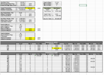
I have created a workbook that is comparing my business transactions from year to year. Each year is represented by a worksheet (2020, 2019, 2018, 2017, etc.). On each worksheet, I have listed the transactions, and then broken down data for the year including number of transactions, total volume, total commission, average sales price, largest transaction, smallest transaction, average # days of a transaction, etc.

I created an "Overall" sheet for the beginning of the workbook to summarize my whole business. I have been able to figure out the formula for the yearly average, the year that had the highest and the year with the lowest of each statistic. But I for the max and the min, I would like that sheet to display which year (or sheet) those stats came from. I can't figure out a formula to display that? I have spent weeks searching the internet for this formula. PLEASE HELP!
 

Excel Facts

What is the shortcut key for Format Selection?
Ctrl+1 (the number one) will open the Format dialog for whatever is selected.
Can you provide Max and Min Formula Here?. I think you can pull sheet name from that formula .
 
Upvote 0
Originally the data points were not in the same cell on each sheet because I have a different number of transactions each year (2014=15 transactions, 2020=41 transactions). But in the process of trying to figure this out, I ended up adding extra rows and hiding them to the sheets with less transactions so that my data analysis each year starts on the same row.

Formula for the Year of Max Transactions:
=MAX('2020'!B61,'2019'!B61,'2018'!B61,'2017'!B61,'2016'!B61,'2015'!B61,'2014'!B61,'2013'!B61)
Answer is 41, which comes from 2020 Sheet

Formula for the Year of Min Transactions:
=MIN('2020'!B61,'2019'!B61,'2018'!B61,'2017'!B61,'2016'!B61,'2015'!B61,'2014'!B61,'2013'!B61)
Answer is 15, which comes from 2014 Sheet

Is that what you were looking for?
 
Upvote 0
Hi! There may be short and efficient Formular! but I could not figure it out.
Try this! Use Ctrl+ Shift+ Enter. this formula is static and absolute if you change some reference cell it won't work!

For Max
Excel Formula:
=MID(SUBSTITUTE(SUBSTITUTE(SUBSTITUTE( ",'2020'!B61,'2019'!B61,'2018'!B61,'2017'!B61,'2016'!B61,'2015'!B61,'2014'!B61,'2013'!B61","'",""),",","@",SUMPRODUCT(IF(CHOOSE({1,2,3,4,5,6,7,8},'2020'!B61,'2019'!B61,'2018'!B61,'2017'!B61,'2016'!B61,'2015'!B61,'2014'!B61,'2013'!B61)=MAX('2020'!B61,'2019'!B61,'2018'!B61,'2017'!B61,'2016'!B61,'2015'!B61,'2014'!B61,'2013'!B61),{1,2,3,4,5,6,7,8}))),"!","#",SUMPRODUCT(IF(CHOOSE({1,2,3,4,5,6,7,8},'2020'!B61,'2019'!B61,'2018'!B61,'2017'!B61,'2016'!B61,'2015'!B61,'2014'!B61,'2013'!B61)=MAX('2020'!B61,'2019'!B61,'2018'!B61,'2017'!B61,'2016'!B61,'2015'!B61,'2014'!B61,'2013'!B61),{1,2,3,4,5,6,7,8}))),FIND("@",SUBSTITUTE(SUBSTITUTE(SUBSTITUTE( ",'2020'!B61,'2019'!B61,'2018'!B61,'2017'!B61,'2016'!B61,'2015'!B61,'2014'!B61,'2013'!B61","'",""),",","@",SUMPRODUCT(IF(CHOOSE({1,2,3,4,5,6,7,8},'2020'!B61,'2019'!B61,'2018'!B61,'2017'!B61,'2016'!B61,'2015'!B61,'2014'!B61,'2013'!B61)=MAX('2020'!B61,'2019'!B61,'2018'!B61,'2017'!B61,'2016'!B61,'2015'!B61,'2014'!B61,'2013'!B61),{1,2,3,4,5,6,7,8}))),"!","#",SUMPRODUCT(IF(CHOOSE({1,2,3,4,5,6,7,8},'2020'!B61,'2019'!B61,'2018'!B61,'2017'!B61,'2016'!B61,'2015'!B61,'2014'!B61,'2013'!B61)=MAX('2020'!B61,'2019'!B61,'2018'!B61,'2017'!B61,'2016'!B61,'2015'!B61,'2014'!B61,'2013'!B61),{1,2,3,4,5,6,7,8}))))+1,FIND("#",SUBSTITUTE(SUBSTITUTE(SUBSTITUTE( ",'2020'!B61,'2019'!B61,'2018'!B61,'2017'!B61,'2016'!B61,'2015'!B61,'2014'!B61,'2013'!B61","'",""),",","@",SUMPRODUCT(IF(CHOOSE({1,2,3,4,5,6,7,8},'2020'!B61,'2019'!B61,'2018'!B61,'2017'!B61,'2016'!B61,'2015'!B61,'2014'!B61,'2013'!B61)=MAX('2020'!B61,'2019'!B61,'2018'!B61,'2017'!B61,'2016'!B61,'2015'!B61,'2014'!B61,'2013'!B61),{1,2,3,4,5,6,7,8}))),"!","#",SUMPRODUCT(IF(CHOOSE({1,2,3,4,5,6,7,8},'2020'!B61,'2019'!B61,'2018'!B61,'2017'!B61,'2016'!B61,'2015'!B61,'2014'!B61,'2013'!B61)=MAX('2020'!B61,'2019'!B61,'2018'!B61,'2017'!B61,'2016'!B61,'2015'!B61,'2014'!B61,'2013'!B61),{1,2,3,4,5,6,7,8}))))-FIND("@",SUBSTITUTE(SUBSTITUTE(SUBSTITUTE( ",'2020'!B61,'2019'!B61,'2018'!B61,'2017'!B61,'2016'!B61,'2015'!B61,'2014'!B61,'2013'!B61","'",""),",","@",SUMPRODUCT(IF(CHOOSE({1,2,3,4,5,6,7,8},'2020'!B61,'2019'!B61,'2018'!B61,'2017'!B61,'2016'!B61,'2015'!B61,'2014'!B61,'2013'!B61)=MAX('2020'!B61,'2019'!B61,'2018'!B61,'2017'!B61,'2016'!B61,'2015'!B61,'2014'!B61,'2013'!B61),{1,2,3,4,5,6,7,8}))),"!","#",SUMPRODUCT(IF(CHOOSE({1,2,3,4,5,6,7,8},'2020'!B61,'2019'!B61,'2018'!B61,'2017'!B61,'2016'!B61,'2015'!B61,'2014'!B61,'2013'!B61)=MAX('2020'!B61,'2019'!B61,'2018'!B61,'2017'!B61,'2016'!B61,'2015'!B61,'2014'!B61,'2013'!B61),{1,2,3,4,5,6,7,8}))))-1)

For MIN!
Excel Formula:
=MID(SUBSTITUTE(SUBSTITUTE(SUBSTITUTE( ",'2020'!B61,'2019'!B61,'2018'!B61,'2017'!B61,'2016'!B61,'2015'!B61,'2014'!B61,'2013'!B61","'",""),",","@",SUMPRODUCT(IF(CHOOSE({1,2,3,4,5,6,7,8},'2020'!B61,'2019'!B61,'2018'!B61,'2017'!B61,'2016'!B61,'2015'!B61,'2014'!B61,'2013'!B61)=MIN('2020'!B61,'2019'!B61,'2018'!B61,'2017'!B61,'2016'!B61,'2015'!B61,'2014'!B61,'2013'!B61),{1,2,3,4,5,6,7,8}))),"!","#",SUMPRODUCT(IF(CHOOSE({1,2,3,4,5,6,7,8},'2020'!B61,'2019'!B61,'2018'!B61,'2017'!B61,'2016'!B61,'2015'!B61,'2014'!B61,'2013'!B61)=MIN('2020'!B61,'2019'!B61,'2018'!B61,'2017'!B61,'2016'!B61,'2015'!B61,'2014'!B61,'2013'!B61),{1,2,3,4,5,6,7,8}))),FIND("@",SUBSTITUTE(SUBSTITUTE(SUBSTITUTE( ",'2020'!B61,'2019'!B61,'2018'!B61,'2017'!B61,'2016'!B61,'2015'!B61,'2014'!B61,'2013'!B61","'",""),",","@",SUMPRODUCT(IF(CHOOSE({1,2,3,4,5,6,7,8},'2020'!B61,'2019'!B61,'2018'!B61,'2017'!B61,'2016'!B61,'2015'!B61,'2014'!B61,'2013'!B61)=MIN('2020'!B61,'2019'!B61,'2018'!B61,'2017'!B61,'2016'!B61,'2015'!B61,'2014'!B61,'2013'!B61),{1,2,3,4,5,6,7,8}))),"!","#",SUMPRODUCT(IF(CHOOSE({1,2,3,4,5,6,7,8},'2020'!B61,'2019'!B61,'2018'!B61,'2017'!B61,'2016'!B61,'2015'!B61,'2014'!B61,'2013'!B61)=MIN('2020'!B61,'2019'!B61,'2018'!B61,'2017'!B61,'2016'!B61,'2015'!B61,'2014'!B61,'2013'!B61),{1,2,3,4,5,6,7,8}))))+1,FIND("#",SUBSTITUTE(SUBSTITUTE(SUBSTITUTE( ",'2020'!B61,'2019'!B61,'2018'!B61,'2017'!B61,'2016'!B61,'2015'!B61,'2014'!B61,'2013'!B61","'",""),",","@",SUMPRODUCT(IF(CHOOSE({1,2,3,4,5,6,7,8},'2020'!B61,'2019'!B61,'2018'!B61,'2017'!B61,'2016'!B61,'2015'!B61,'2014'!B61,'2013'!B61)=MIN('2020'!B61,'2019'!B61,'2018'!B61,'2017'!B61,'2016'!B61,'2015'!B61,'2014'!B61,'2013'!B61),{1,2,3,4,5,6,7,8}))),"!","#",SUMPRODUCT(IF(CHOOSE({1,2,3,4,5,6,7,8},'2020'!B61,'2019'!B61,'2018'!B61,'2017'!B61,'2016'!B61,'2015'!B61,'2014'!B61,'2013'!B61)=MIN('2020'!B61,'2019'!B61,'2018'!B61,'2017'!B61,'2016'!B61,'2015'!B61,'2014'!B61,'2013'!B61),{1,2,3,4,5,6,7,8}))))-FIND("@",SUBSTITUTE(SUBSTITUTE(SUBSTITUTE( ",'2020'!B61,'2019'!B61,'2018'!B61,'2017'!B61,'2016'!B61,'2015'!B61,'2014'!B61,'2013'!B61","'",""),",","@",SUMPRODUCT(IF(CHOOSE({1,2,3,4,5,6,7,8},'2020'!B61,'2019'!B61,'2018'!B61,'2017'!B61,'2016'!B61,'2015'!B61,'2014'!B61,'2013'!B61)=MIN('2020'!B61,'2019'!B61,'2018'!B61,'2017'!B61,'2016'!B61,'2015'!B61,'2014'!B61,'2013'!B61),{1,2,3,4,5,6,7,8}))),"!","#",SUMPRODUCT(IF(CHOOSE({1,2,3,4,5,6,7,8},'2020'!B61,'2019'!B61,'2018'!B61,'2017'!B61,'2016'!B61,'2015'!B61,'2014'!B61,'2013'!B61)=MIN('2020'!B61,'2019'!B61,'2018'!B61,'2017'!B61,'2016'!B61,'2015'!B61,'2014'!B61,'2013'!B61),{1,2,3,4,5,6,7,8}))))-1)
 
Upvote 0
Solution
DANG! That works! Thank you! Can you explain it a little to me? because I am going to have to a) recreate it for like 40 more categories, and b) every year when I add another sheet (another year) I will have to modify it I guess.
 
Upvote 0
Hi! thanks for the feedback.
Here is my explanation at my best.

First part
original Formula range (Answer = 41)
1Ans =MAX('2020'!B61,'2019'!B61,'2018'!B61,'2017'!B61,'2016'!B61,'2015'!B61,'2014'!B61,'2013'!B61)

Remove =Max( )
'2Ans '2020'!B61,'2019'!B61,'2018'!B61,'2017'!B61,'2016'!B61,'2015'!B61,'2014'!B61,'2013'!B61

Place Between ", " ("" Double code to use as text And , Comma for place finder)
'3Ans ",'2020'!B61,'2019'!B61,'2018'!B61,'2017'!B61,'2016'!B61,'2015'!B61,'2014'!B61,'2013'!B61"

SUBSTITUTE ' Single code with ""nothing
=SUBSTITUTE( 3Ans ,"'","")
4Ans ",2020!B61,2019!B61,2018!B61,2017!B61,2016!B61,2015!B61,2014!B61,2013!B61"

Now every sheet name is between , comma and ! (1st sheet is between first , and ! , 2nd sheet is between second , and ! So on…)
Now ,need to know which comma to start and End with !

Second Part
You have Eight sheet name See 2Ans
Use Choose to deliver your eight sheets as range and compare with Max Answer(1Ans) .
{1,2,3,4,5,6,7,8} for eight sheet
5Ans CHOOSE({1,2,3,4,5,6,7,8},'2020'!B61,'2019'!B61,'2018'!B61,'2017'!B61,'2016'!B61,'2015'!B61,'2014'!B61,'2013'!B61)=MAX('2020'!B61,'2019'!B61,'2018'!B61,'2017'!B61,'2016'!B61,'2015'!B61,'2014'!B61,'2013'!B61)
Result Example" Answer is 41, which comes from 2020 Sheet
(41 , 100,200,300,400,500,600,700)= 41
(True , False,False,False,False,False,False,False)

Now Use IF and sumproduct to get location number
If ( 5Ans ,{1,2,3,4,5,6,7,8})
Result example
if((True , False,False,False,False,False,False,False), {1,2,3,4,5,6,7,8} )
Now True will deliver relevent no. which is 1 .and use sumproduct
Sumproduct ( 1) Now you get the answer 1 for which comma to use in first part answer
6Ans 1


Third part
Use Subtitute , and ! With @ and # ( Subtitute can use which instance no to replace)instance no will get from 6Ans
7 Ans


Use Mid to extract sheet name
=MID( 7Ans , find @ from 7 Ans , Find # from 7Ans)
 
Upvote 0
1. It is much more efficient to have all the data on one sheet and the reporting on another. You can use Pivot Tables and a many Excel Formulas.

2. The post below shows a sample of two 3D approaches; the array formula must be array entered (CSE) for versions before 365. I do not know if these work with the Mac version.


2016 3d.xlsm
ABCDEFG
1WorksheetSheets
2ArrayNot CSE2014
3Maximum 24201420142015
4Minimum1201620162016
5
6ArrayNot CSE
7Maximum 2420142014
8Minimum120162016
9
Results
Cell Formulas
RangeFormula
C3,C7C3=MAX('2014:2016'!$A$1:$C$4)
D8,D3:D4D3=INDEX($G$2:$G$4,MATCH(TRUE,COUNTIF(INDIRECT("'"&$G$2:$G$4&"'!A1:C4"),C3)>0,0))
E3E3=INDEX($G$2:$G$4,CEILING(MATCH(1,FREQUENCY(C3,'2014:2016'!$A$1:$C$4),0) / COUNT('2014:2016'!$A$1:$C$4)* COUNTA($G$2:$G$4),1))
C4,C8C4=MIN('2014:2016'!$A$1:$C$4)
E4,E7:E8E4=INDEX(rSheets,CEILING(MATCH(1,FREQUENCY(C4,'2014:2016'!$A$1:$C$4),0) / COUNT('2014:2016'!$A$1:$C$4)* COUNTA(rSheets),1))
D7D7=INDEX(rSheets,MATCH(TRUE,COUNTIF(INDIRECT("'"&rSheets&"'!A1:C4"),C7)>0,0))
Press CTRL+SHIFT+ENTER to enter array formulas.
Named Ranges
NameRefers ToCells
rSheets=Results!$G$2:$G$4D3:E4, D7:E8
 
  • Like
Reactions: alz
Upvote 0
@Dave Patton - Thank you! But the problem is I want to keep the years on separate sheets so I can also look at the entire year.

@alz - I have gone through and plugged in the formula everywhere. It has worked in some places, and has not worked in others. I have attached a screenshot. I highlighted the answer it is showing and then I wrote next to it what the actual answer is. And then it also does #VALUE when the answer is the same on several sheets. Any suggestions?
 

Attachments

  • Screen Shot 2021-01-21 at 12.31.17 PM.png
    Screen Shot 2021-01-21 at 12.31.17 PM.png
    126.2 KB · Views: 29
Upvote 0
Did you try any of the formulas that I suggested?

A participant in the forum will secure more and better suggestions if the extract of data is posted with the forum's tool XL2BB.

2016 3d.xlsm
ABCDEFG
1WorksheetSheets
2ArrayNot CSE2014
3Maximum 24201420142015
4Minimum1201620162016
5
Results
Cell Formulas
RangeFormula
C3C3=MAX('2014:2016'!$A$1:$C$4)
D3:D4D3=INDEX($G$2:$G$4,MATCH(TRUE,COUNTIF(INDIRECT("'"&$G$2:$G$4&"'!A1:C4"),C3)>0,0))
E3E3=INDEX($G$2:$G$4,CEILING(MATCH(1,FREQUENCY(C3,'2014:2016'!$A$1:$C$4),0) / COUNT('2014:2016'!$A$1:$C$4)* COUNTA($G$2:$G$4),1))
C4C4=MIN('2014:2016'!$A$1:$C$4)
E4E4=INDEX(rSheets,CEILING(MATCH(1,FREQUENCY(C4,'2014:2016'!$A$1:$C$4),0) / COUNT('2014:2016'!$A$1:$C$4)* COUNTA(rSheets),1))
Press CTRL+SHIFT+ENTER to enter array formulas.
Named Ranges
NameRefers ToCells
rSheets=Results!$G$2:$G$4D3:E4
 
Upvote 0
@Dave Patton - Thank you! But the problem is I want to keep the years on separate sheets so I can also look at the entire year.

@alz - I have gone through and plugged in the formula everywhere. It has worked in some places, and has not worked in others. I have attached a screenshot. I highlighted the answer it is showing and then I wrote next to it what the actual answer is. And then it also does #VALUE when the answer is the same on several sheets. Any suggestions?

I will not able to suggest without looking at actual Data, ( formula)

you can upload your summary sheets here by using Xl2BB add-in https://www.mrexcel.com/board/excel-articles/xl2bb-excel-range-to-bbcode.1/download
So that, many people can give you better suggestion and write the code directly
 
Upvote 0

Forum statistics

Threads
1,214,374
Messages
6,119,162
Members
448,870
Latest member
max_pedreira

We've detected that you are using an adblocker.

We have a great community of people providing Excel help here, but the hosting costs are enormous. You can help keep this site running by allowing ads on MrExcel.com.
Allow Ads at MrExcel

Which adblocker are you using?

Disable AdBlock

Follow these easy steps to disable AdBlock

1)Click on the icon in the browser’s toolbar.
2)Click on the icon in the browser’s toolbar.
2)Click on the "Pause on this site" option.
Go back

Disable AdBlock Plus

Follow these easy steps to disable AdBlock Plus

1)Click on the icon in the browser’s toolbar.
2)Click on the toggle to disable it for "mrexcel.com".
Go back

Disable uBlock Origin

Follow these easy steps to disable uBlock Origin

1)Click on the icon in the browser’s toolbar.
2)Click on the "Power" button.
3)Click on the "Refresh" button.
Go back

Disable uBlock

Follow these easy steps to disable uBlock

1)Click on the icon in the browser’s toolbar.
2)Click on the "Power" button.
3)Click on the "Refresh" button.
Go back
Back
Top