Formula to extract value from 2 rows below.

[Theocharis]

Hello to everone in the forum.

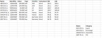
I would like to kindly ask for the expertise and help of someone regarding an important project that I work on in my company. The problem that I am facing is the following: Imagine that I have a dataset similar to sheet1 to the workbook that I attached. I am always receiving bond transactions for the same company always twice indicating one time "Sell" and one time "Buy". The dataset is large with each week around 300 observations coming out. What I need to do is to build a formula so that ONLY ONE of the two cases for each deal either "Sell" or buy but NOT both of them are copied in sheet1 (imagine that it is similar to what I have attached). This means that the formula needs to include only one row of the two that refer to the same company, omit the next one, and move for the next company where it does the same etc. In sheet 2 I also need to extract not the name but the category of the company that issues the bond, which I specify in columns K & L. The formula that I have written in Sheet 2 which apparently doesn't work is the following:

=if(Sheet1!D2="Sell";Vlookup(Sheet1!C2;Sheet1!$K$12:$L$16;2;False);Vlookup(Indirect(Address(Row(Sheet1!C2)+1;Column(Sheet1!C2));Sheet1!$K$12:$L$16;2;False)).

Effectively my intuition is the following: If the cell in column D is "Sell" then go to the table and find me the category, otherwise if the cell in column D is buy, then ommit that row, go to the next one and again take the value from the table specified in columns K and L.

I really struggle to find out what I am doing wrong. Can someone please help me with that one? It would be much appreciated.

Thanks in advance,

Theocharis

 

[earthworm]

In column I input this formula :

=IF(COUNTIF(B$2:B2,B2)=1,1,"-")

In column J input this formula :

=IFERROR(IF(I2="-","-,"-"",SUM(I2:I2)),"-")

In second sheet input serial number 1-100 whatever your length of data is
In second sheet use vlookup / index function to extract data to another sheet using the column J to extract

 

[RoryA]

Please take a minute to read the forum rules on cross-posting and then make sure to follow them in future. Thanks!

Cross-posted here: Formula to extract value from 2 rows below.