Formula To Fill In Days Based On Starting And Ending Dates

[JEF13]

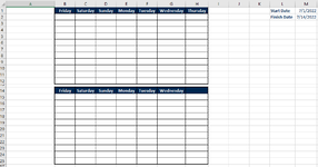
I am looking for a formula that will automatically fill in the day of the week based on the start and end date. The formula is used in a series of cells. Please refer to the screenshot.
As an example, the starting date in L1 is 7/1/2022 and the ending date in L2 is 7/13/2022.

Cell B1 displays Friday
Cell B2 displays Saturday
...
Cell B14 displays Friday
Cell H14 displays nothing

Thank you!

Jeffrey

 

[Ezguy4u]

Jef, Let's get the ball rollin. Now I know you asked for a formula and here is a program, but we have to start some place. So usually this generates more questions than answers so let the discussion begin. If you have any questions let us know.

Sub Prog1()

Dim Date1 As Long
Dim Loop1 As Long
Dim Col1 As Long
Dim Col2 As Long
Dim Add1 As Long

 Range("B2:H2,B14:H14").Select
    Range("B14").Activate
    Selection.Clear
    Range("B2").Select
    
Date1 = Range("M2") - Range("M1")
Row1 = 2

Col1 = 2
Col2 = 2
Add1 = 0

For Loop1 = 2 To Date1 + 2

If Col1 <= 8 Then

    Cells(2, Col1).Select
    Cells(2, Col1).Formula = "=M1" & " +  " & Add1 & ""
    Cells(2, Col1).NumberFormat = "DDDD"
    Col1 = Col1 + 1
    Add1 = Add1 + 1

Else

    Cells(14, Col2).Select
    Cells(14, Col2).Formula = "=M1" & " +  " & Add1 & ""
    Cells(14, Col2).NumberFormat = "DDDD"
    Add1 = Add1 + 1
    Col2 = Col2 + 1

End If

Next Loop1
End Sub

22-06-11 3.xlsm
	B	C	D	E	F	G	H	I	J	K	L	M
1												7/1/2022
2	Friday	Saturday	Sunday	Monday	Tuesday	Wednesday	Thursday					7/11/2022
3
4
5
6
7
8
9
10
11
12
13
14	Friday	Saturday	Sunday	Monday
Date

Cell Formulas
Range	Formula
B2	B2	=M1 + 0
C2	C2	=M1 + 1
D2	D2	=M1 + 2
E2	E2	=M1 + 3
F2	F2	=M1 + 4
G2	G2	=M1 + 5
H2	H2	=M1 + 6
B14	B14	=M1 + 7
C14	C14	=M1 + 8
D14	D14	=M1 + 9
E14	E14	=M1 + 10

 

[JEF13]

Thanks for your time and effort. Much appreciated. I will go through the information nd reach out with any questions!

Thanks.

Jeffrey

 

[Ezguy4u]

Jef, I did some more thinking on your problem and here is a worksheet that just uses a formula to get the results you want. Now the only thing is you have to format the cells using custom format and DDDD.

22-06-11 4.xlsx
	B	C	D	E	F	G	H	I	J	K	L	M	N
1												7/1/2022	Friday, July 1, 2022
2	Friday	Saturday	Sunday	Monday	Tuesday	Wednesday	Thursday					7/10/2022	Sunday, July 10, 2022
3
4
5
6
7
8
9
10
11
12
13
14	Friday	Saturday	Sunday
Date

Cell Formulas
Range	Formula
B2	B2	=IF(M2-M1>= 0,M1 + 0,"")
C2	C2	=IF(M2-M1>= 1,M1 + 1,"")
D2	D2	=IF(M2-M1>= 2,M1 + 2,"")
E2	E2	=IF(M2-M1>= 3,M1 + 3,"")
F2	F2	=IF(M2-M1>= 4,M1 + 4,"")
G2	G2	=IF(M2-M1>= 5,M1 + 5,"")
H2	H2	=IF(M2-M1>= 6,M1 + 6,"")
N1:N2	N1	=M1
B14	B14	=IF(M2-M1>= 7,M1 + 7,"")
C14	C14	=IF(M2-M1>=8,M1 + 8,"")
D14	D14	=IF(M2-M1>=9,M1 + 9,"")
E14	E14	=IF(M2-M1>=10,M1 + 10,"")
F14	F14	=IF(M2-M1>=11,M1 + 11,"")
G14	G14	=IF(M2-M1>=12,M1 + 12,"")
H14	H14	=IF(M2-M1>=13,M1 + 13,"")

 

[JEF13]

Great work on simplifying the solution to be a formula only. Thank you! The new solution is great.

 

[Ezguy4u]

Thanks for the feedback.

 

[JEF13]

Hi everyone. Something has changed with the behavior of the spreadsheet and I'm not sure how to fix it. What's going on is that unless there misinformation of guests up to cell 217 the dates and guest names aren't automatically filled in. So in other words, if the guest list goes up to 84 the system doesn't fill in all 84 guest names. It's only when the guest names go up to 102 does the system fully work. There's been a slight change in the formulas as I put the spreadsheet in Google Sheets for easy team access. Any insights as to how to correct the issues is appreciated. I've pasted the relevant parts of the spread sheet below. Thank you in advance for your help.

Podcast Tracker 2023.xlsx
	A	B	C
1	Guest	Date	Episode
2	Guest 1	Tue 01/03/2023	0191
3	Guest 2	Thu 01/05/2023	0192
4	Guest 3	Tue 01/10/2023	0193
5	Guest 4	Thu 01/12/2023	0194
6	Internal Show 1	Tue 01/17/2023	0195
7	Guest 5	Thu 01/19/2023	0196
8	Guest 6	Tue 01/24/2023	0197
9	Guest 7	Thu 01/26/2023	0198
10	Guest 8	Tue 01/31/2023	0199
11	Internal Show 2	Thu 02/02/2023	0200
12	Guest 9	Tue 02/07/2023	0201
13	Guest 10	Thu 02/09/2023	0202
14	Guest 11	Tue 02/14/2023	0203
15	Guest 12	Thu 02/16/2023	0204
16	Internal Show 3	Tue 02/21/2023	0205
17	Guest 13	Thu 02/23/2023	0206
18	Guest 14	Tue 02/28/2023	0207
19	Guest 15	Thu 03/02/2023	0208
20	Guest 16	Tue 03/07/2023	0209
21	Internal Show 4	Thu 03/09/2023	0210
22	Guest 17	Tue 03/14/2023	0211
23	Guest 18	Thu 03/16/2023	0212
24	Guest 19	Tue 03/21/2023	0213
25	Guest 20	Thu 03/23/2023	0214
26	Internal Show 5	Tue 03/28/2023	0215
27	Guest 21	Thu 03/30/2023	0216
28	Guest 22	Tue 04/04/2023	0217
29	Guest 23	Thu 04/06/2023	0218
30	Guest 24	Tue 04/11/2023	0219
31	Internal Show 6	Thu 04/13/2023	0220
32	Guest 25	Tue 04/18/2023	0221
33	Guest 26	Thu 04/20/2023	0222
34	Guest 27	Tue 04/25/2023	0223
35	Guest 28	Thu 04/27/2023	0224
36	Internal Show 7	Tue 05/02/2023	0225
37	Guest 29	Thu 05/04/2023	0226
38	Guest 30	Tue 05/09/2023	0227
39	Guest 31	Thu 05/11/2023	0228
40	Guest 32	Tue 05/16/2023	0229
41	Internal Show 8	Thu 05/18/2023	0230
42	Guest 33	Tue 05/23/2023	0231
43	Guest 34	Thu 05/25/2023	0232
44	Guest 35	Tue 05/30/2023	0233
45	Guest 36	Thu 06/01/2023	0234
46	Internal Show 9	Tue 06/06/2023	0235
47	Guest 37	Thu 06/08/2023	0236
48	Guest 38	Tue 06/13/2023	0237
49	Guest 39	Thu 06/15/2023	0238
50	Guest 40	Tue 06/20/2023	0239
51	Internal Show 10	Thu 06/22/2023	0240
52	Guest 41	Tue 06/27/2023	0241
53	Guest 42	Thu 06/29/2023	0242
54	Guest 43	Tue 07/04/2023	0243
55	Guest 44	Thu 07/06/2023	0244
56	Internal Show 11	Tue 07/11/2023	0245
57	Guest 45	Thu 07/13/2023	0246
58	Guest 46	Tue 07/18/2023	0247
59	Guest 47	Thu 07/20/2023	0248
60	Guest 48	Tue 07/25/2023	0249
61	Internal Show 12	Thu 07/27/2023	0250
62	Guest 49	Tue 08/01/2023	0251
63	Guest 50	Thu 08/03/2023	0252
64	Guest 51	Tue 08/08/2023	0253
65	Guest 52	Thu 08/10/2023	0254
66	Internal Show 13	Tue 08/15/2023	0255
67	Guest 53	Thu 08/17/2023	0256
68	Guest 54	Tue 08/22/2023	0257
69	Guest 55	Thu 08/24/2023	0258
70	Guest 56	Tue 08/29/2023	0259
71	Internal Show 14	Thu 08/31/2023	0260
72	Guest 57	Tue 09/05/2023	0261
73	Guest 58	Thu 09/07/2023	0262
74	Guest 59	Tue 09/12/2023	0263
75	Guest 60	Thu 09/14/2023	0264
76	Internal Show 15	Tue 09/19/2023	0265
77	Guest 61	Thu 09/21/2023	0266
78	Guest 62	Tue 09/26/2023	0267
79	Guest 63	Thu 09/28/2023	0268
80	Guest 64	Tue 10/03/2023	0269
81	Internal Show 16	Thu 10/05/2023	0270
82	Guest 65	Tue 10/10/2023	0271
83	Guest 66	Thu 10/12/2023	0272
84	Guest 67	Tue 10/17/2023	0273
85	Guest 68	Thu 10/19/2023	0274
86	Internal Show 17	Tue 10/24/2023	0275
87	Guest 69	Thu 10/26/2023	0276
88	Guest 70	Tue 10/31/2023	0277
89	Guest 71	Thu 11/02/2023	0278
90	Guest 72	Tue 11/07/2023	0279
91	Internal Show 18	Thu 11/09/2023	0280
92	Guest 73	Tue 11/14/2023	0281
93	Guest 74	Thu 11/16/2023	0282
94	Guest 75	Tue 11/21/2023	0283
95	Guest 76	Thu 11/23/2023	0284
96	Internal Show 19	Tue 11/28/2023	0285
97	Guest 77	Thu 11/30/2023	0286
98	Guest 78	Tue 12/05/2023	0287
99	Guest 79	Thu 12/07/2023	0288
100	Guest 80	Tue 12/12/2023	0289
101	Internal Show 20	Thu 12/14/2023	0290
102	Guest 81	Thu 12/21/2023	0291
103	Guest 82	Thu 12/28/2023	0292
Master Spreadsheet For Podcast

Cell Formulas
Range	Formula
A2	A2	=IF(B2="","",IF(AND(MOD(ROW()-1,$Q$113)=0,SUMPRODUCT(SIGN(COUNTIF($L$114:$L$199,$A$1:$A1)))<COUNTA($L$114:$L$199)),INDEX($L$114:$L$199,SUMPRODUCT(SIGN(COUNTIF($L$114:$L$199,$A$1:$A1)))+1),INDEX($J$114:$J$199,SUMPRODUCT(SIGN(COUNTIF($J$114:$J$199,$A$1:$A1)))+1)))
A3:A103	A3	=IF(B3="","",IF(AND(MOD(ROW()-1,$Q$113)=0,SUMPRODUCT(SIGN(COUNTIF($L$114:$L$217,$A$1:$A2)))<COUNTA($L$114:$L$217)),INDEX($L$114:$L$217,SUMPRODUCT(SIGN(COUNTIF($L$114:$L$217,$A$1:$A2)))+1),INDEX($J$114:$J$217,SUMPRODUCT(SIGN(COUNTIF($J$114:$J$217,$A$1:$A2)))+1)))
B3:B103	B3	=IF(ROWS(B$2:B3)>COUNTA($J$114:$J$217)+MIN(COUNTA($K$127:$K$217),$M$114),"",WORKDAY.INTL(B2,1,IF(ROWS(B$2:B3)>2*(COUNTA($J$114:$J$217)+MIN(COUNTA($K$127:$K$217),$M$114)-52),"1110111","1010111")))
C3:C103	C3	=IF(LEN(A3)>1,C2+1,"")
Press CTRL+SHIFT+ENTER to enter array formulas.

Cells with Conditional Formatting
Cell	Condition		Cell Format	Stop If True
A2:A112,E113,A200:A1000	Cell Value	contains "Internal"	text	NO

Podcast Tracker 2023.xlsx
	H	I	J	K	L	M	N	O	P	Q
113	Date		Guests	Email	Internal	# of Internal Shows Needed			Number of Internal Shows Every N Weeks	5
114			Guest 1		Internal Show 1	21
115			Guest 2		Internal Show 2
116			Guest 3		Internal Show 3
117			Guest 4		Internal Show 4	Not enough internal shows - filling with guests
118			Guest 5		Internal Show 5
119			Guest 6		Internal Show 6
120			Guest 7		Internal Show 7
121			Guest 8		Internal Show 8
122			Guest 9		Internal Show 9
123			Guest 10		Internal Show 10
124			Guest 11		Internal Show 11
125			Guest 12		Internal Show 12
126			Guest 13		Internal Show 13
127			Guest 14		Internal Show 14
128			Guest 15		Internal Show 15
129			Guest 16		Internal Show 16
130			Guest 17		Internal Show 17
131			Guest 18		Internal Show 18
132			Guest 19		Internal Show 19
133			Guest 20		Internal Show 20
134			Guest 21		Internal Show 21
135			Guest 22
136			Guest 23
137			Guest 24
138			Guest 25
139			Guest 26
140			Guest 27
141			Guest 28
142			Guest 29
143			Guest 30
144			Guest 31
145			Guest 32
146			Guest 33
147			Guest 34
148			Guest 35
149			Guest 36
150			Guest 37
151			Guest 38
152			Guest 39
153			Guest 40
154			Guest 41
155			Guest 42
156			Guest 43
157			Guest 44
158			Guest 45
159			Guest 46
160			Guest 47
161			Guest 48
162			Guest 49
163			Guest 50
164			Guest 51
165			Guest 52
166			Guest 53
167			Guest 54
168			Guest 55
169			Guest 56
170			Guest 57
171			Guest 58
172			Guest 59
173			Guest 60
174			Guest 61
175			Guest 62
176			Guest 63
177			Guest 64
178			Guest 65
179			Guest 66
180			Guest 67
181			Guest 68
182			Guest 69
183			Guest 70
184			Guest 71
185			Guest 72
186			Guest 73
187			Guest 74
188			Guest 75
189			Guest 76
190			Guest 77
191			Guest 78
192			Guest 79
193			Guest 80
194			Guest 81
195			Guest 82
196			Guest 83
197			Guest 84
198			Guest 85
199			Guest 86
200			Guest 87					Guest 87 Guest 88
201			Guest 88
202			Guest 89					Guest 89 Guest 90
203			Guest 90
204			Guest 91					Guest 91 Guest 92
205			Guest 92
206			Guest 93					Guest 93 Guest 94
207			Guest 94
208			Guest 95					Guest 95 Guest 96
209			Guest 96
210			Guest 97					Guest 97 Guest 98
211			Guest 98
212			Guest 99					Guest 99 Guest 100
213			Guest 100
214			Guest 101					Guest 101 Guest 102
215			Guest 102
216
217
Master Spreadsheet For Podcast

Cell Formulas
Range	Formula
M114	M114	=INT((COUNTA(J114:K199)-1)/(Q113-1))
M117	M117	=IF(COUNTA(J114:K199)>104,"Too many shows scheduled for 1 year",IF(COUNTA(K127:K199)<M114,"Not enough internal shows - filling with guests",""))
O200,O216,O214,O212,O210,O208,O206,O204,O202	O200	=IF(J200>0,J200&" "&J201,"")

Cells with Conditional Formatting
Cell	Condition		Cell Format	Stop If True
M113	Expression	=$K113="Y"	text	NO
J117:J127,J130:J139,J143:J152,J156:J165,J169:J172,J176:J186,J189:J224,J228:J231,J235:J245,J248:J257,J261:J270,J274:J283,J287:J290,J294:J304,J307:J316,J320:J329,J333:J342,J346:J349,J353:J363,J366:J373	Cell Value	contains "JeffreyEpisode"	text	NO
L116	Cell Value	contains "JeffreyEpisode"	text	NO
L115,L117,L119,L121,L123,L125,K127,K129,K131,K133,K135,K137,K139,K141,K143,K145	Cell Value	contains "JeffreyEpisode"	text	NO
J135:J139,J194:J215,J253:J257,J312:J316,J371:J373	Cell Value	contains "JeffreyEpisode"	text	NO
J147:J152,J206:J211,J265:J270,J324:J329	Cell Value	contains "JeffreyEpisode"	text	NO
J143:J148,J202:J215,J261:J266,J320:J325	Cell Value	contains "JeffreyEpisode"	text	NO
J140:J144,J199:J203,J258:J262,J317:J321	Cell Value	contains "JeffreyEpisode"	text	NO