Formula to find column value with ticked/filled cells for Google Sheets

[jw2022]

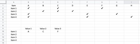
I have a question about what formula I should use for the following:

I have a spreadsheet (similar to below). Across the columns are values such as A, B, C etc. Down the rows are item numbers. I have one table which has these items down the rows and ticks next to the relevant column value. E.g. Item 1 has 'A', 'C' and 'F' ticked. I want to create another table with the rows as the same items, but the columns represent the actual values that have been ticked. Each item has three ticks, so I want the 3 cells to show the 3 values that are ticked. E.g. for Item 2: 'B', 'C' and 'D'.

Is there a formula I can use to find these ticked values to present them in the second table?

 

[nemmi69]

How are the ticks entered?

 

[jw2022]

How are the ticks entered?

The ticks are entered manually and exactly as shown above. Basically across the columns only 3 cells are filled in, the rest are blank.

 

[nemmi69]

is it font Wingding or ASCII 251 or what? Cannot give a formula till we know what the ticks are

 

[jw2022]

is it font Wingding or ASCII 251 or what? Cannot give a formula till we know what the ticks are

In the sheet I am using there are actually two types of ticks ' √ ✓ '

And it is actually a Google Sheets document, so only shows up the default Google fonts.

✓ - Segoe UI Symbol

√ - this is just the system font; which is Calibri

Do I need to reformat the ticks? Or is there not a way to use a formula whereby the values only appear if the cell is not blank?

 

[nemmi69]

In F2

=IF(AND(B2="√",C2="√",D2="√"),"CDE",IF(AND(B2="√",C2="√",D2<>"√"),"BC",IF(AND(B2="√",C2<>"√",D2="√"),"BD",IF(AND(B2<>"√",C2="√",D2="√"),"CD",IF(AND(B2="√",C2<>"√",D2<>"√"),"B",IF(AND(B2<>"√",C2="√",D2<>"√"),"C",IF(AND(B2<>"√",C2<>"√",D2="√"),"D","1")))))))

Then drag down

 

[nemmi69]

Sorry got it wrong, in F2

=IF(AND(B2="√",C2="√",D2="√"),$B$1&$C$1&$D$1,IF(AND(B2="√",C2="√",D2<>"√"),$B$1&$C$1,IF(AND(B2="√",C2<>"√",D2="√"),$B$1&$D$1,IF(AND(B2<>"√",C2="√",D2="√"),$C$1&$D$1,IF(AND(B2="√",C2<>"√",D2<>"√"),$B$1,IF(AND(B2<>"√",C2="√",D2<>"√"),$C$1,IF(AND(B2<>"√",C2<>"√",D2="√"),$D$1,"1")))))))

Allows for any value in B1, C1, D1

 

[jw2022]

View attachment 71425
Sorry got it wrong, in F2

=IF(AND(B2="√",C2="√",D2="√"),$B$1&$C$1&$D$1,IF(AND(B2="√",C2="√",D2<>"√"),$B$1&$C$1,IF(AND(B2="√",C2<>"√",D2="√"),$B$1&$D$1,IF(AND(B2<>"√",C2="√",D2="√"),$C$1&$D$1,IF(AND(B2="√",C2<>"√",D2<>"√"),$B$1,IF(AND(B2<>"√",C2="√",D2<>"√"),$C$1,IF(AND(B2<>"√",C2<>"√",D2="√"),$D$1,"1")))))))

Allows for any value in B1, C1, D1

Thanks for the formula. Actually in my real spreadsheet, I have 30 columns. Using the formula above would be quite tedious, is there another way to achieve this possibly? And also wondering if the values can be in separate cells (as 3 separate values) rather than combined into one cell.

 

[Fluff]

it is actually a Google Sheets document

In future you need to make that clear in your original post & all such questions should be posted to the General Discussion & Other Applications section of the site.
I have done that for you this time.