Formula to find the NEXT to Last Value in a column - minus zeros

[Florida1510]

Excel Gurus,

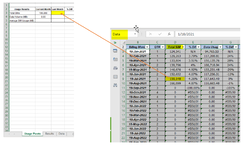
Good morning I need some assistance. I have a results spreadsheet that is feed from another spreadsheet. This results 0.00 in months where there is no data yet. Here is my question I'm trying to find the NEXT to last data field so that my report can show the Current months data and the Previous months data side by side. I have a formula to pull in the last value that is not a zero however I'm struggling to write a formula that will pull in the previous months results. Right since all the future months that have no data are zeros the formula that I have written is going to the bottom of the spreadsheet and pulling in the next to last entry which is a zero. If someone could advise me what I need to add to the below formula so that it will only pull in the previous month result if in has data greater than zero. Note - actual results will always be greater than zero.

Current formula - =INDEX(Data[Total SIMs],AGGREGATE(14,6,(ROW(Data[Total SIMs])-ROW(D3)+1)/(Data[Total SIMs]<>""),2))

I have added an image of my spreadsheet. The result I'm trying to get for this month would be 117,643.40

Any assistance would be appreciated. Thanks in advance.

Owen

 

[Fluff]

Are you trying to get the value from the Total Sims column or the Data Usage column?

 

[Florida1510]

Fluff,

My apologies the screenshot should have pointed to the Total SIMs not the total usage. The results I'm trying to get is 159,148. Sorry about that.

Owen

 

[Fluff]

Ok, thanks for that. How about

=LOOKUP(2,1/(Data[Total SIMs]<>0),Data[[#All],[Total SIMs]])

 

[Florida1510]

Fluff,

That does not seem to work I get this error message

 

[Fluff]

I took the range from the formula you posted. Do you have a table called Data & does it have a column called Total SIMs?

 

[Florida1510]

Fluff

I have attached a screenshot below. In my spreadsheet the Usage Pivots tab in cell L3 is where I need the results. In the Results tab the data table is called Data and the column that the data resides in is in column D "Total SIMs". I'm trying to get the formula to pull in cell D9 from that spreadsheet and put it in Cell L3 on the Usage Pivots tab.

Thanks for all of your help I really appreciate it.

Owen

 

[Fluff]

If the formula you posted works, then the formula I posted should work as it uses the same structured references.