Formula to return last value from list - potential nested If issue

[MarkTheRed]

Hello everyone,

I have what will be a very complex issue (i think), and simply said i do not know how to solve it. Some have adviced VBA, but for reasons of my own i would like to have it in simple formula. Here is an explanation of what is needed. Let's say i have a list of cells with data in it (A1-A5):
1 2 3 4 5

In A6 i need a formula that would always return the data from the last cell (A5), by looking up data from A5 - A1. The catch is that there are times where the values will not be present. Here are some examples:

1 2 3 4 5 - 5
1 3 4 5 - 5
1 1 1 1 1 - 1
3 3 - 3
2 3 - 3

So by looking at these examples, you see that after - i have placed the number that will be the final result in A6, and these examples are some situations that can occur. I have tried using IF with combinations of AND, OR, and i cannot get a proper solution. I know the nested if has the potential to be huge but that is something i will have to live with i guess.

Any assistance would be much appreciated. If someone needs an example in excel (if these are confusing) please let me know.

Thank you

 

[MarkTheRed]

Please bear in mind that, as i've noticed the board does not separate them, any cell from A1-A5 that is empty, would need to be in the calculation, in case at some point data is entered into them.

 

[sandy666]

use XL2BB and post your representative example and expected result

 

[MarkTheRed]

use XL2BB and post your representative example and expected result

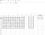
I am unable to install XL2BB, so i have attached a simple image, hope this helps. It should illustrate what i need. The G cells formula should check, starting from E to A, which one contains the "latest" data, and take into consideration empty cells and repeated data.

Thanks

 

[sandy666]

with Power Query

Column1	Column2	Column3	Column4	Column5		Result
1	2	3	4	5		5
1	2	3	4			4
1	2	3				3
1	2			5		5
1			4	4		4
		3	4	1		1
1			1	1		1
2			3	2		2

// Table1
let
    Source = Excel.CurrentWorkbook(){[Name="Table1"]}[Content],
    Merge = Table.CombineColumns(Table.TransformColumnTypes(Source, {{"Column1", type text}, {"Column2", type text}, {"Column3", type text}, {"Column4", type text}, {"Column5", type text}}, "en-GB"),{"Column1", "Column2", "Column3", "Column4", "Column5"},Combiner.CombineTextByDelimiter("", QuoteStyle.None),"Result"),
    LastChar = Table.TransformColumns(Merge, {{"Result", each Text.End(_, 1), type text}})
in
    LastChar

 

[MarkTheRed]

with Power Query

Column1	Column2	Column3	Column4	Column5		Result
1	2	3	4	5		5
1	2	3	4			4
1	2	3				3
1	2			5		5
1			4	4		4
		3	4	1		1
1			1	1		1
2			3	2		2

// Table1
let
    Source = Excel.CurrentWorkbook(){[Name="Table1"]}[Content],
    Merge = Table.CombineColumns(Table.TransformColumnTypes(Source, {{"Column1", type text}, {"Column2", type text}, {"Column3", type text}, {"Column4", type text}, {"Column5", type text}}, "en-GB"),{"Column1", "Column2", "Column3", "Column4", "Column5"},Combiner.CombineTextByDelimiter("", QuoteStyle.None),"Result"),
    LastChar = Table.TransformColumns(Merge, {{"Result", each Text.End(_, 1), type text}})
in
    LastChar

Thank you for this i will test it out. There is a possibility that the cells might be from different sheets, so i will think on how to adapt this, if possible.

 

[sandy666]

example
A1= sheet30!C34
B1= sheet150!D3
etc...
but the result should be like you see in blue table
then you can use Power Query
PQ is designed to work with data not a single cells

just select range,
ribbon - Data - From Table....