Formula to SUM 5 consecutive columns that match a criteria

fchri31

New Member
Joined
Sep 28, 2020
Messages
11
Office Version
  1. 365
Platform
  1. Windows
Hi everyone,

This is my first time using this forum so apologies if this question has been asked before.

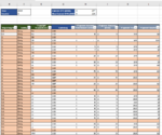
I am trying to create a formula that adds current (within 1 year) accounts and another formula that calculates long term (more than 1 year) accounts.

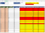
The current accounts are always the 5 consecutive columns from the current year and current quarter. For example, we are in year 2020, Q2. So the current accounts will equal, 2020 Q2 (Column M), 2020 Q3 (Column N), 2020 Q4 (Column O), 2021 Q1 (Column P), 2021 Q2 (Column Q). Next quarter, for Q3, it will be 2020 Q3 (Column N), 2020 Q4 (Column O), 2021 Q1 (Column P), 2021 Q2 (Column Q), 2021 Q3 (Column R)

The long term accounts will always equal the 6th column from the current year and quarter, so in 2020 Q2 case, from 2021 Q3 and onwards.

This formula needs to roll forward, so if I were to update the values in cell C2 and C3, columns H and I should populate for that Quarter and Year's current and long term accounts amounts

There may be an easier way of doing this regarding the format of the excel, so any help would be greatly appreciated. Thank you all for your time.
 

Attachments

  • excel help.PNG
    excel help.PNG
    35.7 KB · Views: 23
Glad to help & thanks for the feedback.
 
Upvote 0

Excel Facts

Quick Sum
Select a range of cells. The total appears in bottom right of Excel screen. Right-click total to add Max, Min, Count, Average.
Hi again,

Thank you for your help above, but I was wondering you could assist again with something similar. So we are still using the original formula you provided us as a check, but we wanted to recreate the format of the file. The format now looks like the attached picture, in which Column I contains the pertinent amount that we want to be summed, Column K contains the Year, and Column L contains the Quarter. Cell C2 and C3 represent which current and noncurrent amounts we are looking for and we hope that when we change this, it will update the values. For example, if we were trying to sum for all current amounts in Q3 2020, it will sum column I for all the following quarters: Q3 2020, Q4 2020, Q1 2021, Q2 2021, and Q3 2021. This sum will represent the current amounts. If were to change C3 to "4" we would hope it would sum the Q4 2020, Q1 2021, Q2 2021, Q3 2021, and Q4 2021 amounts. We hope that this current amount can be displayed in cell H2.

For the non-current amounts, it will equal Q4 2021 through Q4 2026 if C3 is "3". If C3 is "4", it will equal Q1 2022 through Q4 2026. We hope that this non-current amount can be displayed in cell H3.

Our data currently goes down to row 69.

Thank you again for all your help, it is truly appreciated.
 

Attachments

  • Excel help 3.PNG
    Excel help 3.PNG
    33.3 KB · Views: 5
Upvote 0
How about
Excel Formula:
=SUM(FILTER(I8:I100,(K8:K100&L8:L100>=C2&"Q"&C3)*(K8:K100&L8:L100<=C2+1&"Q"&C3)))
=SUM(FILTER(I8:I100,K8:K100&L8:L100>=C2+1&"Q"&C3+1))
 
Upvote 0
Hey Fluff,

Thank you for all your help before and now. So after using the formula, I am getting a total that seems to be incorrect. Please see attached picture (I filtered for 2020 and onwards) where I have highlighted yellow the amounts that would be considered current and highlighted orange the amounts that should be considered noncurrent based on Q3 2020 and totaled these two amounts. As you can see, it results in a different amount than what the formula is creating. Not quite sure if you know why, but as always, your helps is greatly appreciated.
 

Attachments

  • Excel help 4.PNG
    Excel help 4.PNG
    38.6 KB · Views: 5
Upvote 0
Can you post some sample data using the XL2BB add-in, it's impossible to test with an image. ;)
 
Upvote 0
Playing around with it, It seems that it is pulling Q4 2021 into as non current, but it should be considered current!
 
Upvote 0
Here you are. I hope I did it right! Thanks!!

for fluff.xlsx
BCEGHIKL
2Year2020Current DTS (USD)256.72364Yellow sum (Current)$ 296.72
3Quarter3Non Current DTS (USD)225Orange sum (Noncurrent)$ 185
4Red highlighted is irrelevant
5
6
7Reporting UnitEntityCopyright AcquisitionsCurrencyPayment Amount Functional CurrencyPayment Amount (USD)Payment YearPayment Quarter
23SEntityGGGBP£ 34$ 44.392020Q1
25SEntityHHGBP£ 20$ 26.112020Q2
27SEntityIIUSD$ 44$ 44.002020Q2
30NSEntityJJUSD$ 10$ 10.002020Q1
31NSEntityJJUSD$ 10$ 10.002021Q1
32NSEntityJJUSD$ 10$ 102022Q1
33NSEntityJJUSD$ 10$ 102023Q1
34NSEntityJJUSD$ 10$ 102024Q1
35NSEntityJJUSD$ 10$ 102025Q1
36NSEntityJJUSD$ 15$ 152026Q1
39NSEntityLLUSD$ 25$ 25.002020Q3
41NSEntityMMUSD$ 30$ 30.002020Q2
42NSEntityMMUSD$ 40$ 40.002020Q2
44SEntityNNUSD$ 50$ 50.002020Q1
48SEntityPPGBP£ 40$ 52.222020Q2
50SEntityQQUSD$ 60$ 60.002021Q3
51SEntityQQUSD$ 70$ 702022Q3
53SEntityRRUSD$ 43$ 43.002021Q2
55SEntitySSGBP£ 22$ 28.722021Q1
57NSEntityTTUSD$ 10$ 10.002020Q2
58NSEntityTTUSD$ 10$ 10.002020Q3
59NSEntityTTUSD$ 10$ 10.002020Q4
60NSEntityTTUSD$ 10$ 10.002021Q1
61NSEntityTTUSD$ 10$ 10.002021Q2
62NSEntityTTUSD$ 10$ 10.002021Q3
63NSEntityTTUSD$ 10$ 10.002021Q4
64NSEntityTTUSD$ 20$ 202022Q1
66SEntityUUUSD$ 30$ 30.002021Q4
68SEntityVVUSD$ 40$ 40.002021Q3
69SEntityVVUSD$ 40$ 402022Q3
Current v Non Current
Cell Formulas
RangeFormula
H2H2=SUM(FILTER(I8:I100,(K8:K100&L8:L100>=C2&"Q"&C3)*(K8:K100&L8:L100<=C2+1&"Q"&C3)))
H3H3=SUM(FILTER(I8:I100,K8:K100&L8:L100>=C2+1&"Q"&C3+1))
K2K2=SUM(I31+I39+I50+I53+I55+I58+I59+I60+I61+I62+I63+I66+I68)
K3K3=SUM(I32:I36)+I51+I64+I69
I23I23=H23*O8
I25I25=H25*O8
I27,I68:I69,I64,I57:I62,I53,I50:I51,I44,I41:I42,I39,I30:I36I27=H27*1
I48I48=H48*O8
I55I55=H55*O8
 
Upvote 0
You said that if you had 2020 & 3 it should sum Q3 2020, Q4 2020, Q1 2021, Q2 2021, and Q3 2021
Which is what it is doing.
 
Upvote 0
Hi Fluff,

My apologies, you are correct. It was an issue on my end as to why I thought the formula wasn't working.

Thank you again for everything, you truly are a life saver and are the best!!!
 
Upvote 0
You're welcome & thanks for the feedback.
 
Upvote 0

Forum statistics

Threads
1,214,591
Messages
6,120,426
Members
448,961
Latest member
nzskater

We've detected that you are using an adblocker.

We have a great community of people providing Excel help here, but the hosting costs are enormous. You can help keep this site running by allowing ads on MrExcel.com.
Allow Ads at MrExcel

Which adblocker are you using?

Disable AdBlock

Follow these easy steps to disable AdBlock

1)Click on the icon in the browser’s toolbar.
2)Click on the icon in the browser’s toolbar.
2)Click on the "Pause on this site" option.
Go back

Disable AdBlock Plus

Follow these easy steps to disable AdBlock Plus

1)Click on the icon in the browser’s toolbar.
2)Click on the toggle to disable it for "mrexcel.com".
Go back

Disable uBlock Origin

Follow these easy steps to disable uBlock Origin

1)Click on the icon in the browser’s toolbar.
2)Click on the "Power" button.
3)Click on the "Refresh" button.
Go back

Disable uBlock

Follow these easy steps to disable uBlock

1)Click on the icon in the browser’s toolbar.
2)Click on the "Power" button.
3)Click on the "Refresh" button.
Go back
Back
Top