Formula with IF & And if Blank then 0

[Yogesh977]

Dear Expert,

Please help me with below formula in not able to capture formula if cell one cell or both cell is blank. for reference Image with formula attached and sheet as below

i need you help please help me if its possible for you all experts.
Thank for your support.

	A	B	C	D	E	F	G	H	I	J	K
1​	Status	Sr.No.	My Tax Number	Vendor Tax Number	Product Amt	Tax %	Central Tax @9%	State Tax @9%	Integrated Tax @18%	Total Invoice Amt	Remark
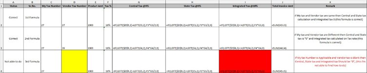
2​	Correct	1st Formula	27	27	1000	18%	90	90	0	180	if My tax and Vendor tax are same then Central and State tax calculation and Integrated tax 0 (this formula is correct)
3​	Correct	2nd Formula	27	26	1000	18%	0	0	180	180	if My tax and Vendor tax are Different then Central and State tax is "0" and Integrated tax calculated on Tax rate (this formula is correct)
4​	Not able to do	3rd Formula	27		1000	18%	0	0	180	180	if My tax Number is Applicable and Vendor tax is Blank then Central, State tax and Integrated tax Should be "0", (this I'm not able to find how to do)

 

[maabadi]

Please Use XL2BB to upload your example file. Also Show Cell D9.

 

[Nishant94]

24.11.2020.xlsx
A
B
C
D
E
F
G
H
I
J
1
Status
Sr.No.
My Tax Number
Vendor Tax Number
Product Amt
Tax %
Central Tax @9%
State Tax @9%
Integrated Tax @18%
Total Invoice Amt
2
Correct
1st Formula
18AABCU9603R1ZM
18AABCU9603R1Z2
1000
18%
90
90
0
180
3
Correct
2nd Formula
10AABCU9603R1Z2
04AABCU9603R1ZV
1000
18%
0
0
180
180
4
Not able to do
3rd Formula
22AABCU9603R1ZX
1000
18%
0
0
0
0
Sheet1
Cell Formulas
Range
Formula
I2:I4
I2
=IF(LEFT(C2,2)<>LEFT(D2,2),(E2*F2)*(1-(SUM(--(C2:D2=""))>0)),0)
J2:J4
J2
=SUM(Sheet1!$G2:$I2)

 

[maabadi]

This Part of Your formula is array and you use SHIFT+CTRL+ENTER not ENTER:
SUM(--(C3:D3=""))

Also I don't see how your last Row formula take data from one lower row ( No data).

 

[maabadi]

In I4 You can Write (change Your formula to what you want):

=IF(AND(C4<>"",D4=""),0,Your Formula)

and drag it up and down if needed

 

[Nishant94]

This Part of Your formula is array and you use SHIFT+CTRL+ENTER not ENTER:
SUM(--(C3:D3=""))

Also I don't see how your last Row formula take data from one lower row ( No data).

I guess he is using office 365 as he has mentioned in his profile. In that case, even a normal ENTER would work.

However, if he isn't then he will have to use SHIFT+CTRL+ENTER.

 

[Yogesh977]

Thank to all of you for your kind reply and support my be my explanations is not correct please refer this one
my Concern is my all formula is working fine what i want my only difficulty is if Vendor Tax Number is Blank then nothing to be calculated in Central,state, Integrated and show 0 value

Note:
I want red highlighted to be 0 value after my formula (if Vendor Tax Number is Blank then nothing is calculated in Central,state, Integrated)
1st Formula : IF My Tax Number and Vendor Tax Number Is Same Then Central Tax & State Tax is calculate and integrated tax should not calculate
2nd Formula :IF My Tax Number and Vendor Tax Number Is Different Then Central Tax & State Tax Should calculate 0 or blank and integrated should calculate
3rd Formula : if Vendor Tax Number is Blank then nothing to be calculated in Central,state, Integrated

GST Formula.xlsx
	A	B	C	D	E	F	G	H	I	J	K	L	M	N
1	Status	Sr.No.	My Tax Number	Vendor Tax Number	Product Amt	Tax %	Central Tax @9%	State Tax @9%	Integrated Tax @18%	Total Invoice Amt
2	Correct	1st Formula	18AABCU9603R1ZM	18AABCU9603R1Z2	1000	18%	90	90	0	1180
3	Correct	2nd Formula	18AABCU9603R1Z2	04AABCU9603R1ZV	1000	18%	0	0	180	1180
4	Not able to do	3rd Formula	18AABCU9603R1Z2		1000	18%	0	0	180	1180
5
6	want like this	3rd Formula	18AABCU9603R1Z2		1000	18%	0	0	0	1000	Manual amount done need in formula
7
8
9
Sheet2

Cell Formulas
Range	Formula
G2:G4	G2	=IF(LEFT(C2,2)=LEFT(D2,2),E2*F2/2,0)
H2:H4	H2	=IF(LEFT(C2,2)=LEFT(D2,2),E2*F2/2,0)
I2:I4	I2	=IF(LEFT(C2,2)<>LEFT(D2,2),E2*F2,0)
J6,J2:J4	J2	=SUM(G2:I2)+E2

 

[maabadi]

Change I2 to this and drag it down:

=IF(OR(LEFT(C2,2)<>LEFT(D2,2),D2="",C2=""),E2*F2,0)

this is for if Column C or D is blank. if you want only for D use this

=IF(OR(LEFT(C2,2)<>LEFT(D2,2),D2=""),E2*F2,0)

 

[Yogesh977]

Change I2 to this and drag it down:

=IF(OR(LEFT(C2,2)<>LEFT(D2,2),D2="",C2=""),E2*F2,0)

this is for if Column C or D is blank. if you want only for D use this

=IF(OR(LEFT(C2,2)<>LEFT(D2,2),D2=""),E2*F2,0)

Not Working

GST Formula.xlsx
	A	B	C	D	E	F	G	H	I	J
1	Status	Sr.No.	My Tax Number	Vendor Tax Number	Product Amt	Tax %	Central Tax @9%	State Tax @9%	Integrated Tax @18%	Total Invoice Amt
2	Correct	1st Formula	18AABCU9603R1ZM	18AABCU9603R1Z2	1000	18%	90	90	0	1180
3	Correct	2nd Formula	18AABCU9603R1Z2	04AABCU9603R1ZV	1000	18%	0	0	180	1180
4	Not able to do	3rd Formula	18AABCU9603R1Z2		1000	18%	0	0	180	1180
Sheet2

Cell Formulas
Range	Formula
G2:G4	G2	=IF(LEFT(C2,2)=LEFT(D2,2),E2*F2/2,0)
H2:H4	H2	=IF(LEFT(C2,2)=LEFT(D2,2),E2*F2/2,0)
I2:I4	I2	=IF(OR(LEFT(C2,2)<>LEFT(D2,2),D2="",C2=""),E2*F2,0)
J2:J4	J2	=SUM(G2:I2)+E2

 

[maabadi]

Sorry My fault:

=IF(OR(D2="",C2=""),0,IF(LEFT(C2,2)<>LEFT(D2,2),E2*F2,0)