Function to pull table data by two parameters

[8thwondurrrr]

Hello,
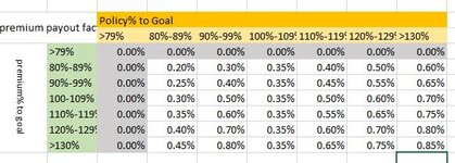
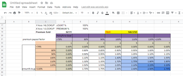
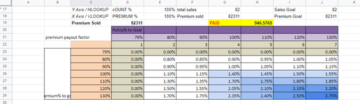
I am looking for help creating a tracker for commissions earned, first looking up premium % to goal in a Column and then returning the cell input for a corresponding row for the policy% count to goal. I had the attached table starting in Cell q1, and the formula to find the multiplier (table data) is as follows
=(vlookup(e3,r4:y10,hlookup(e2,s2:y3,2,false),false)).
in this function e3 is where the tracker is calculating the sold premiums % to goal and e2 is the % to count goals.

As an idea, on if you made 100% to goal for premium and count, the function should return .35% multiplier.

We need the function to be able to work inside a range of percentages. Any Ideas???

Thank you in advance!

 

[GraH]

Can you share some sample data? Preferably using XL2BB. Makes it easier to help you.
At first glance, I would use an INDEX-Match-Match combo.
Maybe the % goals on top and the left could be Bins (80% , 90%, 100%, ...) as it is easier to find approximate matches.
Using a match("Premium", RangeOfGoals,0) + match("%, RangeOf%,0) enables finding the correct % over multiple partitions inside a single "table".

 

[8thwondurrrr]

I apologize for whatever the reason the add in isn't working I'll try to provide some additional details.
In the example, we have 100% to Premium and 100% to count, so the multiplier should be 1.40, meaning my formula should calculate $1,152.354 ($82,311 * 1.40) but instead it is calculating $946 (Looks like it is multiplying $82,311 * 1.15%).

Here is my Formula:
=D19*(VLOOKUP(E18,C23:J29,HLOOKUP(E17,D21:J22,2,FALSE),FALSE))

I attached the screenshot for reference.

 

[Toadstool]

Hi 8thwondurrrr,

Your HLOOKUP returns 4 and as your VLOOKUP starts in column C it will retrieve F26.

You will have other challenges as your first and last boundaries horizontally and vertically start "<" or ">" so the cell is treated as text, which is why it left aligns by default.

 

[8thwondurrrr]

Thank you for the help, even when I remove the less than or greater than symbols remove it still doesn't calculate correctly.
Also, how can I make the spreadsheet use the correct columns and rows when the % to goal is not an exact match. IE if you are at lets say 99% it will use the 90% column/row?

 

[Toadstool]

Does this do what you want?

8thwondurrrr.xlsx
	B	C	D	E	F	G	H	I	J
17			Y HLOOKUP	100%
18			X VLOOKUP	100%
19		Premium sold	82311			PAID	1152.354
20			Policty2goal
21	Premium payout factor		0%	80%	90%	100%	110%	120%	130%
22			1	2	3	4	5	6	7
23		0%	0.00%	0.00%	0.00%	0.00%	0.00%	0.00%	0.00%
24		80%	0.00%	0.80%	0.85%	0.90%	0.95%	1.00%	1.05%
25		90%	0.00%	0.90%	0.95%	1.00%	1.05%	1.10%	1.15%
26		100%	0.00%	1.10%	1.15%	1.40%	1.45%	1.50%	1.55%
27		110%	0.00%	1.30%	1.35%	1.70%	1.75%	1.80%	1.85%
28		120%	0.00%	1.50%	1.55%	2.05%	2.10%	2.15%	2.20%
29		130%	0.00%	1.70%	1.75%	2.35%	2.40%	2.50%	2.75%
Sheet1

Cell Formulas
Range	Formula
H19	H19	=D19*(VLOOKUP(E18,C23:J29,1+HLOOKUP(E17,D21:J22,2,TRUE),TRUE))

 

[8thwondurrrr]

Yes! Adding the 1+ works, so does changing row H to start at 2 (instead of 1). Great thank you!

How can I make it to where the it works on a range of cells instead of only the percent's in row 21? IE it will work is we are at lets say 80%, but not 81% or 82%.

 

[Toadstool]

Yes! Adding the 1+ works, so does changing row H to start at 2 (instead of 1). Great thank you!

How can I make it to where the it works on a range of cells instead of only the percent's in row 21? IE it will work is we are at lets say 80%, but not 81% or 82%.

Did you try on the sheet I supplied? Changing FALSE to TRUE for the HLOOKUP and VLOOKUP should do what you ask.

 

[8thwondurrrr]

THANK ALL OF YOU SO MUCH!!!!!!!!!!!