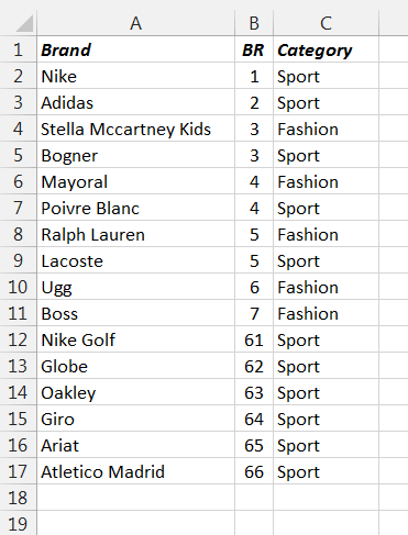
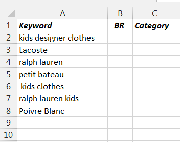
I have two sheets in Excel 2013: One contains more than 200 Brandnames, plus their importance on an increasing scale starting at 1, plus a category. The second sheetcontains more than 13,000 keyword phrases, which may – or may not – contain the Brandnames in the first table.
What I want to do is to use a sort of VLOOKUP() statement to search Sheet 1 for each of the 13,000 keywords in Sheet 2 and – if it finds a partial match – return the Importance and Category.
For example ...
Result for "Ralph Lauren kids"
Because the actual numbers of results are too large to show here, I've created a test book to show the actual problem.
Sheet1
Sheet2
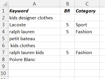
In a perfect world, the end result should be ...
Sheet2
I found what I believed was a solution elsewhere on this forum; however, despite modifying the formula given there for Sheet2/C7 to read ...
... it still doesn't work.
I've also run it past our office Excel guru and he's stumped too, so I'm wondering if this really is a solution after all.
I'd be grateful for any help. I could do it manually, but 13,000 lines of updates is a very long weekend.")
Thanks in advance,
m
What I want to do is to use a sort of VLOOKUP() statement to search Sheet 1 for each of the 13,000 keywords in Sheet 2 and – if it finds a partial match – return the Importance and Category.
For example ...
Keyword = "Ralph Lauren kids";
Brand = "Ralph Lauren"
Brand = "Ralph Lauren"
Brand-Importance = "124"
Brand-Category = "Fashion"
Brand-Category = "Fashion"
Result for "Ralph Lauren kids"
Keyword-Importance = "124"
Keyword-Category = "Fashion"
Keyword-Category = "Fashion"
Because the actual numbers of results are too large to show here, I've created a test book to show the actual problem.
Sheet1
Sheet2
In a perfect world, the end result should be ...
Sheet2
I found what I believed was a solution elsewhere on this forum; however, despite modifying the formula given there for Sheet2/C7 to read ...
Code:
=IF(ISNA(LOOKUP(10^10,FIND(Sheet2!$A$1:$C$17,A7),Sheet2!$B$2:$B$6)),"",LOOKUP(10^10,FIND(Sheet2!$A$2:$A$6,A7),Sheet2!$B$2:$B$6))... it still doesn't work.
I've also run it past our office Excel guru and he's stumped too, so I'm wondering if this really is a solution after all.
I'd be grateful for any help. I could do it manually, but 13,000 lines of updates is a very long weekend.
Thanks in advance,
m


