GENERATING AN EMAIL FOR EACH SHEET (insert sheet data between 2 sentences of email body)

JuicyMusic

Board Regular
Joined
Jun 13, 2020
Messages
210
Office Version
  1. 365
Platform
  1. Windows
Good Mooring,

I have been using a code that splits data from the "Source" tab into separate sheets. Each new sheet that is created ends up having the employee name as the sheet name - based on names in column A (starting at cell A3)

I need a code that will generate an email for each employee that has a new sheet. The number of new sheets will vary but never over 35 or so though, in case that is important.
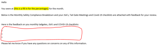
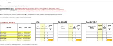
The data from column A thru Z (thru to the last row of data) will need to be inserted in between the 4th and 5th sentence of a stock email from PR. I will provide the email template below. Every one will get the same wording.

The data set for each generated email should appear where I've indicated with a red rectangle on the 1st uploaded image. The user will be getting each employee's email address themselves.
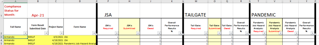
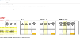
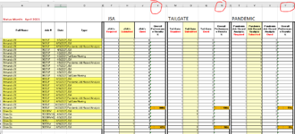
the 2nd image is of the Source tab. I'm sorry that I can't upload this correctly. My company won't allow it.


"Source" tab specifics:
1) Row 1 has the report name and reporting month in cell A1 and B1
2) Row 2 has the headers - from column A thru Z
3) Column E & L & S & Z have no data in them. They are just highlighted black to visually separate 3 sections for data entry. For visual ease only.
4) Column G & I, and N & P, and U & W are hidden columns that contain helper formulas. They will always be hidden.
5) Each data set on each new tab has the exact number of columns - but the number of rows per new sheet WILL vary.

Thank you so much in advance,
Juicy
 

Attachments

  • Capture_Stock Email Template.PNG
    Capture_Stock Email Template.PNG
    15.9 KB · Views: 16
  • Capture_Source tab data.PNG
    Capture_Source tab data.PNG
    28.6 KB · Views: 14
Instead of highlighting the columns in black, you could try removing the color and formatting the right and left borders of each column with a thick black border.
 
Upvote 0

Excel Facts

Shade all formula cells
To shade all formula cells: Home, Find & Select, Formulas to select all formulas. Then apply a light fill color.
Hi, I did what you asked and here is what the email looks like now.

Is it possible to keep the Autofit formatting on the transfer? The data in the first thru fourth columns are being cut off. We are so close!!!
 

Attachments

  • Capture_1 generated email_no black columns.PNG
    Capture_1 generated email_no black columns.PNG
    48.1 KB · Views: 7
Upvote 0
To be honest, I'm not sure what is happening. The "autofit" line of code should be adjusting all the column widths. It is hard to suggest a possible solution without working with the actual file. I f you de-sensitize the data, could you upload a copy of your file to a free site such as www.box.com or www.dropbox.com. Once you do that, mark it for 'Sharing' and you will be given a link to the file that you can post here. I wouldn't need all the data, just 5 or six rows so I can test the macro. Make sure that the de-sensitized file is an exact representation of your actual file.
 
Upvote 0
Mumps, it looks like it's transferring data up to 9 digits only. I counted the the digits of the EE name, job #, date, and form name.

Do you see that too?

I'm asking my IT department if I can to the www.box.com
 
Upvote 0
See if this fixes the problem:
VBA Code:
Sub Split_Data_Into_Tabs()
    Dim lr As Long, ws As Worksheet, vcol, i As Integer, icol As Long, myarr As Variant, title As String, titlerow As Integer
    Dim OutApp As Object, OutMail As Object, rng As Range
    'This macro splits data into multiple worksheets based on the variables on a column found in Excel.
    'An InputBox asks you which columns you'd like to filter by, and it just creates these worksheets.
    Application.ScreenUpdating = False
    vcol = Application.InputBox(prompt:="Which column would you like to filter by?", title:="Filter column", Default:="3", Type:=1)
    Set ws = ActiveSheet
    lr = ws.Cells(ws.Rows.Count, vcol).End(xlUp).Row
    title = "A1"
    titlerow = ws.Range(title).Cells(1).Row
    icol = ws.Cells(1, Columns.Count).End(xlToLeft).Column + 1
    ws.Cells(1, icol) = "Unique"
    For i = 2 To lr
        On Error Resume Next
        If ws.Cells(i, vcol) <> "" And Application.WorksheetFunction.Match(ws.Cells(i, vcol), ws.Columns(icol), 0) = 0 Then
            ws.Cells(ws.Rows.Count, icol).End(xlUp).Offset(1) = ws.Cells(i, vcol)
        End If
    Next
    myarr = Application.WorksheetFunction.Transpose(ws.Columns(icol).SpecialCells(xlCellTypeConstants))
    ws.Columns(icol).Clear
    Set OutApp = CreateObject("Outlook.Application")
    For i = 2 To UBound(myarr)
        ws.Range(title).AutoFilter field:=vcol, Criteria1:=myarr(i) & ""
        If Not Evaluate("=ISREF('" & myarr(i) & "'!A1)") Then
            Sheets.Add(After:=Worksheets(Worksheets.Count)).Name = myarr(i) & ""
            ws.Range("A" & titlerow & ":A" & lr).EntireRow.Copy Sheets(myarr(i) & "").Range("A1")
            Sheets(myarr(i) & "").Columns.AutoFit
            Set rng = Sheets(myarr(i) & "").UsedRange
            Set OutMail = OutApp.CreateItem(0)
            With OutMail
                .To = ""
                .Subject = ""
                .HTMLBody = "You were at (percentage) for the month." & "<br><br>" & "Below is the Monthly Safety Compliance Breakdown " & _
                    "and your ISA's. Tailgate Meetings and COVID-19 checklists are attached with feedback for your review." _
                    & "<br><br>" & "Here is the feedabck on your monthly tailgates, ISA's and COVID-19 checklists:" & "<br><br>" _
                    & RangetoHTML(rng) & "<br><br>" & "Please let me know if you have any questions or concerns on any of this information."
                .Display
            End With
        Else
            Sheets(myarr(i) & "").Move After:=Worksheets(Worksheets.Count)
            ws.Range("A" & titlerow & ":A" & lr).EntireRow.Copy Sheets(myarr(i) & "").Range("A1")
        End If
    Next i
    ws.AutoFilterMode = False
    ws.Activate
    Application.ScreenUpdating = True
End Sub

Function RangetoHTML(rng As Range)
    Dim fso As Object
    Dim ts As Object
    Dim TempFile As String
    Dim TempWB As Workbook
    TempFile = Environ$("temp") & "\" & Format(Now, "dd-mm-yy h-mm-ss") & ".htm"
    rng.Copy
    Set TempWB = Workbooks.Add(1)
    With TempWB.Sheets(1)
        .Cells(1).PasteSpecial Paste:=8
        .Cells(1).PasteSpecial xlPasteValues, , False, False
        .Cells(1).PasteSpecial xlPasteFormats, , False, False
        .Cells(1).Select
        Application.CutCopyMode = False
        On Error Resume Next
        .DrawingObjects.Visible = True
        .DrawingObjects.Delete
        On Error GoTo 0
    End With
    With TempWB.PublishObjects.Add( _
         SourceType:=xlSourceRange, _
         Filename:=TempFile, _
         Sheet:=TempWB.Sheets(1).Name, _
         Source:=TempWB.Sheets(1).UsedRange.Address, _
         HtmlType:=xlHtmlStatic)
        .Publish (True)
    End With
    Set fso = CreateObject("Scripting.FileSystemObject")
    Set ts = fso.GetFile(TempFile).OpenAsTextStream(1, -2)
    RangetoHTML = ts.readall
    ts.Close
    RangetoHTML = Replace(RangetoHTML, "align=center x:publishsource=", "align=left x:publishsource=")
    TempWB.Close savechanges:=False
    Kill TempFile
    Set ts = Nothing
    Set fso = Nothing
    Set TempWB = Nothing
End Function
 
Upvote 0
Solution
Good Mooring Mumps, IT WORKED PERFECTLY! Thank you so much. I am amazed as always with your work.
I do have an additional request but I wasn't sure if I should put it on a separate thread . I'll write it here so you can read it and tell me if I should create a new post.

QUESTION: Is it possible to insert three new phrases into the body of the email - that will reflect the percentages for each category below. See the orange and bold cells, for example.
The color coding for the overall percentage results is due to a conditional formatting and may be either Yellow, Orange, or Red.

I've attached an example image for you, and the red text is what I'm writing to you.

The three additional phrases will be as follows (for this example):

Performance Results for JSA: 67%
Performance Results for TAILGATE: 50%
Performance Results for PANDEMIC: 11%


Thank you!!
 

Attachments

  • Capture_Insert percentages from below__to above.PNG
    Capture_Insert percentages from below__to above.PNG
    64.3 KB · Views: 9
Upvote 0
Inserting the text and percentages would not be a problem. I could also make the percentage bold fairly easily. However, getting the color of the overall percentage results would be fairly complicated because the color is a result of conditional formatting so I don't think that I would be able to format the color. If you are happy with the rest, I would need to know in which columns and rows the three results are found.
 
Upvote 0
Mumps, I can live without the colors. Yes, please. The percentage results appear in columns K , R, and Y - at the last row of data based on the name change in column A.

I've added an image of the data source tab so you can see. Thank you! Excited!!!
 

Attachments

  • Capture_ColumnK & R & Y on data source tab.PNG
    Capture_ColumnK & R & Y on data source tab.PNG
    69 KB · Views: 7
Upvote 0
Try:
VBA Code:
Sub Split_Data_Into_Tabs()
    Dim lr As Long, ws As Worksheet, vcol, i As Integer, icol As Long, myarr As Variant, title As String, titlerow As Integer
    Dim OutApp As Object, OutMail As Object, rng As Range, lVisRow As Long
    'This macro splits data into multiple worksheets based on the variables on a column found in Excel.
    'An InputBox asks you which columns you'd like to filter by, and it just creates these worksheets.
    Application.ScreenUpdating = False
    vcol = Application.InputBox(prompt:="Which column would you like to filter by?", title:="Filter column", Default:="3", Type:=1)
    Set ws = ActiveSheet
    lr = ws.Cells(ws.Rows.Count, vcol).End(xlUp).Row
    title = "A1"
    titlerow = ws.Range(title).Cells(1).Row
    icol = ws.Cells(1, Columns.Count).End(xlToLeft).Column + 1
    ws.Cells(1, icol) = "Unique"
    For i = 2 To lr
        On Error Resume Next
        If ws.Cells(i, vcol) <> "" And Application.WorksheetFunction.Match(ws.Cells(i, vcol), ws.Columns(icol), 0) = 0 Then
            ws.Cells(ws.Rows.Count, icol).End(xlUp).Offset(1) = ws.Cells(i, vcol)
        End If
    Next
    myarr = Application.WorksheetFunction.Transpose(ws.Columns(icol).SpecialCells(xlCellTypeConstants))
    ws.Columns(icol).Clear
    Set OutApp = CreateObject("Outlook.Application")
    For i = 2 To UBound(myarr)
        ws.Range(title).AutoFilter field:=vcol, Criteria1:=myarr(i) & ""
        lVisRow = ws.Cells(ws.Rows.Count, "A").End(xlUp).Row
        If Not Evaluate("=ISREF('" & myarr(i) & "'!A1)") Then
            Sheets.Add(After:=Worksheets(Worksheets.Count)).Name = myarr(i) & ""
            ws.Range("A" & titlerow & ":A" & lr).EntireRow.Copy Sheets(myarr(i) & "").Range("A1")
            Sheets(myarr(i) & "").Columns.AutoFit
            Set rng = Sheets(myarr(i) & "").UsedRange
            Set OutMail = OutApp.CreateItem(0)
            With OutMail
                .To = ""
                .Subject = ""
                .htmlBody = "These are the percentages for the month shown below:" & "<br><br>" _
                    & "Performance Results for JSA:  " & ws.Range("K" & lVisRow) & "<br>" _
                    & "Performance Results for TAILGATE:  " & ws.Range("R" & lVisRow) & "<br>" _
                    & "Performance Results for PANDEMIC:  " & ws.Range("Y" & lVisRow) & "<br><br>" _
                    & "Below is the Monthly Safety Compliance Breakdown " & _
                    "and your ISA's. Tailgate Meetings and COVID-19 checklists are attached with feedback for your review." _
                    & "<br><br>" & "Here is the feedabck on your monthly tailgates, ISA's and COVID-19 checklists:" & "<br><br>" _
                    & RangetoHTML(rng) & "<br><br>" & "Please let me know if you have any questions or concerns on any of this information."
                .Display
            End With
        Else
            Sheets(myarr(i) & "").Move After:=Worksheets(Worksheets.Count)
            ws.Range("A" & titlerow & ":A" & lr).EntireRow.Copy Sheets(myarr(i) & "").Range("A1")
        End If
    Next i
    ws.AutoFilterMode = False
    ws.Activate
    Application.ScreenUpdating = True
End Sub
Function RangetoHTML(rng As Range)
    Dim fso As Object
    Dim ts As Object
    Dim TempFile As String
    Dim TempWB As Workbook
    TempFile = Environ$("temp") & "\" & Format(Now, "dd-mm-yy h-mm-ss") & ".htm"
    rng.Copy
    Set TempWB = Workbooks.Add(1)
    With TempWB.Sheets(1)
        .Cells(1).PasteSpecial Paste:=8
        .Cells(1).PasteSpecial xlPasteValues, , False, False
        .Cells(1).PasteSpecial xlPasteFormats, , False, False
        .Cells(1).Select
        Application.CutCopyMode = False
        On Error Resume Next
        .DrawingObjects.Visible = True
        .DrawingObjects.Delete
        On Error GoTo 0
    End With
    With TempWB.PublishObjects.Add( _
         SourceType:=xlSourceRange, _
         Filename:=TempFile, _
         Sheet:=TempWB.Sheets(1).Name, _
         Source:=TempWB.Sheets(1).UsedRange.Address, _
         HtmlType:=xlHtmlStatic)
        .Publish (True)
    End With
    Set fso = CreateObject("Scripting.FileSystemObject")
    Set ts = fso.GetFile(TempFile).OpenAsTextStream(1, -2)
    RangetoHTML = ts.readall
    ts.Close
    RangetoHTML = Replace(RangetoHTML, "align=center x:publishsource=", "align=left x:publishsource=")
    TempWB.Close savechanges:=False
    Kill TempFile
    Set ts = Nothing
    Set fso = Nothing
    Set TempWB = Nothing
End Function
 
Upvote 0

Forum statistics

Threads
1,214,827
Messages
6,121,809
Members
449,048
Latest member
greyangel23

We've detected that you are using an adblocker.

We have a great community of people providing Excel help here, but the hosting costs are enormous. You can help keep this site running by allowing ads on MrExcel.com.
Allow Ads at MrExcel

Which adblocker are you using?

Disable AdBlock

Follow these easy steps to disable AdBlock

1)Click on the icon in the browser’s toolbar.
2)Click on the icon in the browser’s toolbar.
2)Click on the "Pause on this site" option.
Go back

Disable AdBlock Plus

Follow these easy steps to disable AdBlock Plus

1)Click on the icon in the browser’s toolbar.
2)Click on the toggle to disable it for "mrexcel.com".
Go back

Disable uBlock Origin

Follow these easy steps to disable uBlock Origin

1)Click on the icon in the browser’s toolbar.
2)Click on the "Power" button.
3)Click on the "Refresh" button.
Go back

Disable uBlock

Follow these easy steps to disable uBlock

1)Click on the icon in the browser’s toolbar.
2)Click on the "Power" button.
3)Click on the "Refresh" button.
Go back
Back
Top