Get 2nd entry from array (with a criterion)

[virtuosok]

Hi,
I am posting a clip from a large spreadsheet below... headers take up the first 5 rows so the data starts from row 6 downwards.
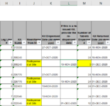
Focus is on kit re-dispensations (column L), ignoring direct dispensations in column K. I'm not showing columns A-G as these are patient identifiers.
I have XLOOKUP set up to identify first kit re-dispensed on a given date for a given patient, so for my first patient, and re-dispensation date 10-NOV-2020 (see column L), I'm getting 208240 from column I. So far, so good.
The question is, how can I pull re-dispensed kit number #2 on the same date? In other words, can I have a formula tagging to kit #1 (208240) as a reference point and pull me kit #2 from the same date in column L (10 Nov 2020), which is kit # 226776? My problem is that dispensation and re-dispensation dates are all thrown together in a random sequence I can't just assume next entry in the spreadsheet.

 

[Peter_SSs]

For the other two formulas, unfortunately they don't seem to be working for me - I am getting #N/A error.

Tricky to resolve for sure since you have only provided a picture (not actual data) of part of the relevant data. In particular, your formula refers to C4 and FULL_1!$E$6:$E$10000 and we have no information about those, not even a picture.

At this stage my best guess is that those two ranges contain numerical data but one of them is actual numeric and the other is 'number stored as text'. Is that possible? If so, which is which?

If that is not the case then can you give us a small set of sample dummy data (sensitive information changed) with XL2BB ?

 

[virtuosok]

Tricky to resolve for sure since you have only provided a picture (not actual data) of part of the relevant data. In particular, your formula refers to C4 and FULL_1!$E$6:$E$10000 and we have no information about those, not even a picture.

At this stage my best guess is that those two ranges contain numerical data but one of them is actual numeric and the other is 'number stored as text'. Is that possible? If so, which is which?

If that is not the case then can you give us a small set of sample dummy data (sensitive information changed) with XL2BB ?

Thank you Peter_SSs,
Especially for patience with my data representation...
Yes your assumption is correct, C4 is a (4-digit) number whereas FULL_1!$E$6:$E$10000 is the set of 4-digit numbers stored as text.

 

[Peter_SSs]

C4 is a (4-digit) number whereas FULL_1!$E$6:$E$10000 is the set of 4-digit numbers stored as text.

If you want all rows from the kit column that meet the criteria then try the next formula. Note that this would replace the need for the above formula.

=FILTER(Full_1!I6:I10000,(Full_1!E6:E10000=C4)*(Full_1!L6:L10000=SUBSTITUTE(G3," ","-")),NA())

If you specifically want the second occurrence only then try

=INDEX(FILTER(Full_1!I6:I10000,(Full_1!E6:E10000=C4)*(Full_1!L6:L10000=SUBSTITUTE(G3," ","-")),{"#N/A","#N/A"}),2)

In that case my suggestions above change just slightly

If you want all rows ..
=FILTER(Full_1!I6:I10000,(Full_1!E6:E10000=C4&"")*(Full_1!L6:L10000=SUBSTITUTE(G3," ","-")),NA())

For specifically the second occurrence only
=INDEX(FILTER(Full_1!I6:I10000,(Full_1!E6:E10000=C4&"")*(Full_1!L6:L10000=SUBSTITUTE(G3," ","-")),{"","#N/A"}),2)

 

[virtuosok]

OMG both are working perfectly, THANK YOU Peter_SSs, this helps immensely!

 

[virtuosok]

...if possible, could you please also explain what does the red bit at the end mean?
=FILTER(Full_1!I6:I10000,(Full_1!E6:E10000=C4&"")*(Full_1!L6:L10000=SUBSTITUTE(G3," ","-")),NA())

 

[Peter_SSs]

THANK YOU Peter_SSs, this helps immensely!

You're welcome. Glad it worked for you.

what does the red bit at the end mean?

It means that if there are no rows in 'Full_1' that meet the criteria, a #N/A error will result.
If you prefer, you could replace that with just "" or a message in quotes like "Nothing found"