Get the max sum of 2 or more consecutive values

[sama9000]

I'm either looking for a formula solution or vba code to calculate the data on cells L2 and M2 ( I've tried multiple formulas and I cant accomplish what I need)

Explanation

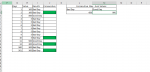
I've a table from column range G:I, the table is registering the days from 1 to 1000, the value is the amount sold ( it can be a credit or debit) , when is a Credit, column "I" will display "Good Day", otherwise "Bad day" for debits. All of this calculation is being processed correctly, the problem comes when I want to get the max sum value for either the consecutive "Good Days" or "Bad Days"

Day 1 and Day 2 are consecutive "Bad Days" and the sum of both values is 200 ( so far this is the maximum sum value ), the problem comes when I get again consecutive "Bad Days" and the sum of those values is greater than my initial consecutive max sum values. Day 500 and 501 are consecutive "Bad Days" and the sum of both is 600 ( that is what I want in cell L2). The same process for "Good Day"

Consecutive days mean more than 1 day either being "Bad Day" or "Good Day" , example, 2 days,4 days, 100 days,etc. Let's say I've got 100 consecutive "Bad Days" with a sum of 1000 , then I got 1 "God Day" and then I got 2 consecutive "Bad Days" with a sum of 5000 which is greater than the one I've got in the 100 consecutive "Bad days" before ( I will need the 5000 value on cell L2)

On the picture below, the first 2 days are consecutive "Bad days" and the total sum is 200 ( so far this is the max value). From day 4 to day 10 there 7 consecutive "Bad Days" and the total sum is 35 ( which is less than the total of previous consecutive values which was 200). Now Days 500 and 501 are 2 consecutive "Bad Days" and the total sum is 600 which is greater than the previous 2 consecutive days on day 1 and 2. 600 will be now my max value that I need on cell L2 ( if someone change the results or values, L2 must be updated too

 

[jasonb75]

I'm assuming that column J is just something that you've added to the example which will not normally be there.

The easiest way would be with 2 helper columns,
In J2 and fill down =IF(AND(I2<>I3,I2="Bad Day"),SUMIFS(H$2:H2,I$2:I2,"Bad Day")-SUM(J$1:J1),"")
In K2 and fill down =IF(AND(I2<>I3,I2="Good Day"),SUMIFS(H$2:H2,I$2:I2,"Good Day")-SUM(K$1:K1),"")

Then the 'Bad day' result will be = MAX(J:J) and 'Good day' result will be =MAX(K:K)

With excel 2019, you could get it down to 1 helper column or with office 365 it might be possible to do it without helpers.
It could be done without helpers in 2016 but the formulas will be far more complex and inefficient.

 

[jasonb75]

Following up on my first reply, I had a go at doing this without the helper columns. This works with the example provided, but I haven't tested it beyond that.

Book2 12-8-20.xlsm
	G	H	I	J	K	L	M
1	Days	Value	Results
2	1	100	Bad Day			Bad Day	Good Day
3	2	100	Bad Day			600	800
4	3	500	Good Day
5	4	5	Bad Day
6	5	5	Bad Day
7	6	5	Bad Day
8	7	5	Bad Day
9	8	5	Bad Day
10	9	5	Bad Day
11	10	5	Bad Day
12	11	500	Good Day
13	12	300	Good Day
14	500	300	Bad Day
15	501	300	Bad Day
Sheet6

Cell Formulas
Range	Formula
L3:M3	L3	=MAX(IFNA(SUBTOTAL(9,OFFSET($H$2,AGGREGATE(15,6,(ROW($I$2:$I$15)-ROW($I$2))/($I$2:$I$15=L$2)/($I$1:$I$14<>L$2),ROW(INDIRECT("1:"&COUNTIFS($I$2:$I$15,L$2,$I$1:$I$14,"<>"&L$2)))),0,FREQUENCY(IF($I$2:$I$15=L$2,ROW($I$2:$I$15)),IF($I$2:$I$15<>L$2,IF($I$1:$I$14=L$2,ROW($I$2:$I$15)))),1)),""))
Press CTRL+SHIFT+ENTER to enter array formulas.

 

[jasonb75]

I realised that the formulas in my earlier posts were not looking for 2 or more consecutive days and that single rows would be included in the results. I've edited the single cell formula to work with that, but haven't had chance to do the helper column one. I'll have another look at that later if you would prefer that method for simplicity.

Book2 12-8-20.xlsm
	G	H	I	J	K	L	M
1	Days	Value	Results
2	1	100	Bad Day			Bad Day	Good Day
3	2	100	Bad Day			600	800
4	3	1000	Good Day
5	4	5	Bad Day
6	5	5	Bad Day
7	6	5	Bad Day
8	7	5	Bad Day
9	8	5	Bad Day
10	9	5	Bad Day
11	10	5	Bad Day
12	11	500	Good Day
13	12	300	Good Day
14	500	300	Bad Day
15	501	300	Bad Day
Sheet6

Cell Formulas
Range	Formula
L3:M3	L3	=MAX(IFERROR(SUBTOTAL(9,OFFSET($H$2,AGGREGATE(15,6,(ROW($I$2:$I$15)-ROW($I$2))/($I$2:$I$15=L$2)/($I$3:$I$16=L$2)/($I$1:$I$14<>L$2),ROW(INDIRECT("1:"&COUNTIFS($I$2:$I$15,L$2,$I$3:$I$16,L$2,$I$1:$I$14,"<>"&L$2)))),0,1/(1/FREQUENCY(IF(($I$2:$I$15=L$2)*($I$1:$I$14=L$2),ROW($I$2:$I$15)),IF($I$3:$I$16<>L$2,IF($I$2:$I$15=L$2,IF($I$1:$I$14=L$2,ROW($I$2:$I$15))))))+1,1)),""))
Press CTRL+SHIFT+ENTER to enter array formulas.

 

[sama9000]

I realised that the formulas in my earlier posts were not looking for 2 or more consecutive days and that single rows would be included in the results. I've edited the single cell formula to work with that, but haven't had chance to do the helper column one. I'll have another look at that later if you would prefer that method for simplicity.

Book2 12-8-20.xlsm
	G	H	I	J	K	L	M
1	Days	Value	Results
2	1	100	Bad Day			Bad Day	Good Day
3	2	100	Bad Day			600	800
4	3	1000	Good Day
5	4	5	Bad Day
6	5	5	Bad Day
7	6	5	Bad Day
8	7	5	Bad Day
9	8	5	Bad Day
10	9	5	Bad Day
11	10	5	Bad Day
12	11	500	Good Day
13	12	300	Good Day
14	500	300	Bad Day
15	501	300	Bad Day
Sheet6

Cell Formulas
Range	Formula
L3:M3	L3	=MAX(IFERROR(SUBTOTAL(9,OFFSET($H$2,AGGREGATE(15,6,(ROW($I$2:$I$15)-ROW($I$2))/($I$2:$I$15=L$2)/($I$3:$I$16=L$2)/($I$1:$I$14<>L$2),ROW(INDIRECT("1:"&COUNTIFS($I$2:$I$15,L$2,$I$3:$I$16,L$2,$I$1:$I$14,"<>"&L$2)))),0,1/(1/FREQUENCY(IF(($I$2:$I$15=L$2)*($I$1:$I$14=L$2),ROW($I$2:$I$15)),IF($I$3:$I$16<>L$2,IF($I$2:$I$15=L$2,IF($I$1:$I$14=L$2,ROW($I$2:$I$15))))))+1,1)),""))
Press CTRL+SHIFT+ENTER to enter array formulas.

Thank you so much for your help , this gave me the solution I needed to build the formula