Getting a 00-Jan-00 when using index match referring to a blank cell

[Fuzzy]

I have a large spreadsheet used to record the date of training for a number of individuals. Their names are to the left of the spreadsheet, as is their occupation, and the dates for each course are in the next columns ( and am currently using 20 columns. Each individual will not necessarily attempt all courses (depending upon occupation) therefore a number of cells will not have a date in them.
I have to create a 'form' which references the spreadsheet for the OHS guys to get a ready readout of individuals.
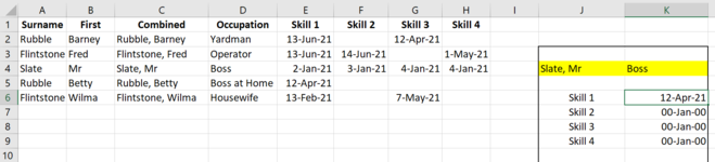
I have created a drop down (data validation) for columns C and D and they are (for this exercise) in J4 and K4 respectively.
I have used the index match formula but am getting a 00-Jan-00, or incorrect date in the cells K6, K7, K8 and K9 I have used ={(INDEX(A2:H6,MATCH(1,(C:C=J4)*(D:D=K4),0),5))} (5 being the column number)
Obviously, I doing something quite incorrectly and any assistance will be appreciated.
Thanking you in advance
Fuzzy

 

[jasonb75]

An empty cell has a value of zero which is why you get 00-Jan-00 in some cells. Also, you need to have the same number of rows in the index and match ranges, otherwise it creates an offset.

Array confirm this in K6 then fill down, no need to manually change for each skill. There are other ways of doing it, I've based this on your original attempt so that you can follow it easier.

=IFERROR(1/(1/INDEX($E$2:$H$6,MATCH(1,($C$2:$C$6=$J$4)*($D$2:$D$6=$K$4),0),MATCH($J6,$E$1:$H$1,0))),"")

 

[Fuzzy]

An empty cell has a value of zero which is why you get 00-Jan-00 in some cells. Also, you need to have the same number of rows in the index and match ranges, otherwise it creates an offset.

Array confirm this in K6 then fill down, no need to manually change for each skill. There are other ways of doing it, I've based this on your original attempt so that you can follow it easier.

=IFERROR(1/(1/INDEX($E$2:$H$6,MATCH(1,($C$2:$C$6=$J$4)*($D$2:$D$6=$K$4),0),MATCH($J6,$E$1:$H$1,0))),"")

I works and thanking you very much. I appreciated you stayed with my 'original attempt' as it makes it a lot easier to understand 'why it works'
Again, thanks and good night
Fuzzy