Getting information from multiple sheets

quintin

Board Regular
Joined
Jun 26, 2013
Messages
52
Good day,
Regular excel
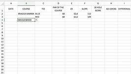
I am needing assistance with the following issues. I have three sheets with data in them, the first one has a list of golf courses, the second has the courses (the name, par, slope, rating). On the third sheet is where I would like to enter the data as I played. Col A the date, col B a drop-down menu with a list of the courses, col C which tee, col D par of the course, col E the course rating, col F the slope. Thereafter are col’s that need to be filled in, in order to complete your round, and then at the end, you’ll be able to work out other information and handicap.

I am needing assistance with col’s c,d,e &f. so that once you select the course in the drop-down menu and selecting the color tee in col c, it should put the rest of the information from the other sheets into the blank spaces.

It goes down for 20 enters, from this I would then be able to work out other info.

I have tried the if function, index, match, and others, but I'm not sure.

I thank you for any assistance in advance.

Quintin
 

Excel Facts

Format cells as currency
Select range and press Ctrl+Shift+4 to format cells as currency. (Shift 4 is the $ sign).
Hi Quintin,

I'm not sure if I followed you correctly so let me just give you my example sheets.

Names of Courses
Quintin.xlsx
A
1Course
2Pebble Beach
3PitchnPutt
4St Andrews
5Mike Pitch&Putt
6Carl Crazy Golf
7
Names


Course details for each tee
Quintin.xlsx
ABCDE
1NameTeeParRatingSlope
2PitchnPutt12D22
3PitchnPutt22D12
4Pebble Beach14A3
5Pebble Beach23B2
6Pebble Beach35D5
7Pebble Beach45A2
8Pebble Beach55C2
9Pebble Beach64A3
10Pebble Beach75C4
11Pebble Beach85D2
12Carl Crazy Golf15A2
13Carl Crazy Golf25B2
14Carl Crazy Golf34C3
15Carl Crazy Golf45D4
16Mike Pitch&Putt15D2
17
Courses


Games sheet where you enter the Date in A2, select Course Name from dropdown in B2 and the formulae fill in 20 rows of columns C,D,E and F.

Quintin.xlsx
ABCDEFGHIJKL
1DateCourseTeeParCourse RatingSlopeStrokes PlayedStrokes RecordedBalls LostClubs BrokenNo. Clubs Thrown into LakeAmount Owed to Swear Jar
205-Jan-21Carl Crazy Golf15A2
325B2
434C3
545D4
6    
7    
8    
9    
10    
11    
12    
13    
14    
15    
16    
17    
18    
19    
20    
21    
Games
Cell Formulas
RangeFormula
C2:F21C2=IFERROR(INDEX(Courses!B$2:B$9999,AGGREGATE(15,6,ROW(Courses!$A$2:$A$9999)-ROW(Courses!$A$1)/(Courses!$A$2:$A$9999=$B$2),ROW()-ROW($C$1))),"")
Cells with Data Validation
CellAllowCriteria
B2List=OFFSET(Names!$A$2,,,COUNTA(Names!$A$2:$A$99))
 
Upvote 0
Thank you for the formula's, I did everything as you have explained. However, I can only put info in the first cell B2, thereafter you are able to use the drop-down menu but, no information is placed in the other cells. Find attached screen shot.
Many thanks
 

Attachments

  • Image 2021-01-17 at 16.30.jpeg
    Image 2021-01-17 at 16.30.jpeg
    62.4 KB · Views: 9
Upvote 0
I thought with maximum 20 rows you were going to just do one course at a time.
For the rows where there is no Course Name I need some reference after the first row. If there's always two tees for a course, or you only play one course a day and the date is repeated for every row where you expect data then I can figure something out.

Can you share the other sheets using XL2BB
 
Upvote 0
Its works however, what I would like it to do is.

Col A is date

Col B is course (which is a drop-down menu)

Col C is the tee you would be teeing off from.

So once you have chosen your course, then in the next col C you would then have to choose (eg on which course colors may vary) See example

Course one Tee Red par of the course 68 course rating 62,4 slope 112

Course one Tee blue par of the course 68 course rating 61,4 slope 109

Other course may have up to four tee off areas.

Once you have selected the color tee then it should put the relevant information into col’s D (par of the course), E (course rating) and E (slope)


On a separate worksheet I have a list of the courses and etc

Col A course

Col B tees

Col C par of the course

Col D rating

Col E slope

Eg col A col B Col C Col D Col E

course one Tee red par of the course course rating slope

course one tee blue par of the course course rating slope

course two tee green par of the course course rating slope

course two tee blue par of the course course rating slope

and so it goes on with a total of 13 courses, however, the list is made up of 42, meaning that most of the courses have more than 2 tee off colors, the most been 4 tee off areas/colors.

I hope this makes more sense and must apologies for not been clear in the beginning.
Thank you
Quintin
 
Upvote 0
OK, here's my amended Courses data sheet
Quintin.xlsx
ABCDE
1NameTeeParRatingSlope
2PitchnPuttRed29D111
3PitchnPuttGreen27D112
4Pebble BeachRed7278145
5Pebble BeachGreen7075.5144
6Pebble BeachBlue7177143
7Pebble BeachWhite6976142
8Pebble BeachYellow7175141
9Pebble BeachGold7274140
10Carl Crazy GolfRed3266122
11Carl Crazy GolfGreen2955123
12Carl Crazy GolfBlue3044124
13Carl Crazy GolfWhite3133125
14Mike Pitch&PuttGreen192899
Courses


Here's the amended Games sheet. The formula in cell D2 can be copied right into E2 and F2 then D2:F2 can be copied down as many fields as you want.

Quintin.xlsx
ABCDEFGHI
1DateCourseTeePar of the CourseCRSlope18 Hole ScoreAdj GrossDifferential
205-Jan-21Pebble BeachGreen7075.5144
3Yellow7175141
4Blue7177143
5White6976142
606-Jan-21PitchnPuttRed29D111
708-Jan-21Mike Pitch&PuttGreen192899
8    
9   
Games
Cell Formulas
RangeFormula
D2:F9D2=IFERROR(INDEX(Courses!C$2:C$999, MATCH(1, INDEX(((INDEX($B$2:$B$99,AGGREGATE(14,6,ROW($B$2:$B$99)-ROW($B$1)/(($B$2:$B$99<>"")*(ROW($B$2:$B$99)<=ROW())),1)))=Courses!$A$2:$A$9997) * ($C2=Courses!$B$2:$B$999), 0, 1), 0)),"")
C8C8=IFERROR(INDEX(Courses!B$2:B$9997,AGGREGATE(15,6,ROW(Courses!$A$2:$A$9997)-ROW(Courses!$A$1)/(Courses!$A$2:$A$9997=$B$2),ROW()-ROW($C$1))),"")
Cells with Data Validation
CellAllowCriteria
B2:B9List=OFFSET(Names!$A$2,,,COUNTA(Names!$A$2:$A$99))


NOTES:
1. You may want to lock the formulae cells as they're in the middle of your data entry area.
2. If a Tee is selected which is not valid for the course then no data is retrieved.
 
Upvote 0
Solution
Good day,
I would just like to thank you for your patience, and your assistance.
I know a few things about excel, but there is always room for improvement.
Thank You
Quintin
 
Upvote 0
You're welcome!
...and please ignore the formula in C8 as it was left over from a previous iteration.
 
Upvote 0

Forum statistics

Threads
1,214,584
Messages
6,120,385
Members
448,956
Latest member
JPav

We've detected that you are using an adblocker.

We have a great community of people providing Excel help here, but the hosting costs are enormous. You can help keep this site running by allowing ads on MrExcel.com.
Allow Ads at MrExcel

Which adblocker are you using?

Disable AdBlock

Follow these easy steps to disable AdBlock

1)Click on the icon in the browser’s toolbar.
2)Click on the icon in the browser’s toolbar.
2)Click on the "Pause on this site" option.
Go back

Disable AdBlock Plus

Follow these easy steps to disable AdBlock Plus

1)Click on the icon in the browser’s toolbar.
2)Click on the toggle to disable it for "mrexcel.com".
Go back

Disable uBlock Origin

Follow these easy steps to disable uBlock Origin

1)Click on the icon in the browser’s toolbar.
2)Click on the "Power" button.
3)Click on the "Refresh" button.
Go back

Disable uBlock

Follow these easy steps to disable uBlock

1)Click on the icon in the browser’s toolbar.
2)Click on the "Power" button.
3)Click on the "Refresh" button.
Go back
Back
Top