Hi Everyone!
I am trying to create a spreadsheet to better track equipment as well as personnel at work.
The basic idea is managers at different sites submit daily a check list at that info is added to a sheet similar to my sample.
 docs.google.com
However, I am trying to figure out how to easily identify the following
1. Who/ what is not currently being used and is available
2. Is anyone/ anything being accidentally double booked?
3. Who/ what needs to move job sites
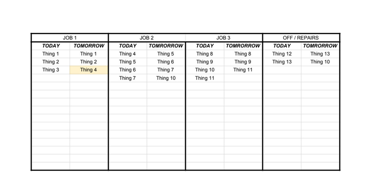
So in my sample
- Thing four is moving from job 2 to job 1 tomorrow.
- Thing 3 is available tomorrow
- Thing 10 is being scheduled when it should be off for repairs.
I'm not asking someone to do this all for me I'm more trying to bounce ideas around. In reality, there are about 20 jobs, 100 employees, and 200 pieces of equipment so it is a lot more data than the sample.
To show moving from one job to another
- I was also trying conditional formatting =countif($A3:$A17,"<>"&B3), this highlights everything so that doesn't work
To show something available
- I honestly don't know on this one.
Things I was trying
To solve locating duplicates, like how thing 10 is off and on job 2 tomorrow
- I was trying to use conditional formatting for a combination of if the name in row 2 is "today" countif($A$3:$H$17,A3)>1)) but wasn't having much luck with that.
I am trying to create a spreadsheet to better track equipment as well as personnel at work.
The basic idea is managers at different sites submit daily a check list at that info is added to a sheet similar to my sample.
Sample
Sheet1 JOB 1,JOB 2,JOB 3,OFF / REPAIRS TODAY,TOMORROW,TODAY,TOMRORROW,TODAY,TOMRORROW,TODAY,TOMRORROW Thing 1,Thing 1,Thing 4,Thing 5,Thing 8,Thing 8,Thing 12,Thing 13 Thing 2,Thing 2,Thing 5,Thing 6,Thing 9,Thing 9,Thing 13,Thing 10 Thing 3,Thing 4,Thing 6,Thing 7,Thing 10,Thing 11 Thing 7,Thin...
However, I am trying to figure out how to easily identify the following
1. Who/ what is not currently being used and is available
2. Is anyone/ anything being accidentally double booked?
3. Who/ what needs to move job sites
So in my sample
- Thing four is moving from job 2 to job 1 tomorrow.
- Thing 3 is available tomorrow
- Thing 10 is being scheduled when it should be off for repairs.
I'm not asking someone to do this all for me I'm more trying to bounce ideas around. In reality, there are about 20 jobs, 100 employees, and 200 pieces of equipment so it is a lot more data than the sample.
To show moving from one job to another
- I was also trying conditional formatting =countif($A3:$A17,"<>"&B3), this highlights everything so that doesn't work
To show something available
- I honestly don't know on this one.
Things I was trying
To solve locating duplicates, like how thing 10 is off and on job 2 tomorrow
- I was trying to use conditional formatting for a combination of if the name in row 2 is "today" countif($A$3:$H$17,A3)>1)) but wasn't having much luck with that.


