diversification
New Member
- Joined
- Jun 24, 2020
- Messages
- 37
- Office Version
- 365
- Platform
- Windows
Hello,
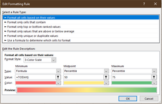
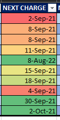
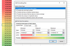
I'm trying to conditionally format a column that's filled with due dates. I'd like it to to be conditionally formatted with a 3-color gradient starting at yellow, moving to orange, and finally to red. I'd like the fill to begin with yellow when the due date in the cell is about 10 days away, then progress to be fully orange sometime around the 5-day-away mark, and then becoming fully red once the due date has arrived or passed. I'm not really certain where to start with with his one. Dates in the date column are formatted as DD/MM/YYYY if that matters.
I would like to avoid any VBA code - I haven't gotten into that stuff yet. Thanks!