Graph Showing Staff Away over holiday period + how many away from each team

[VirtualInsanity]

Hi there,

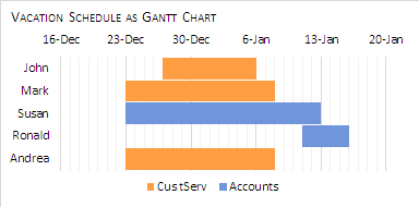
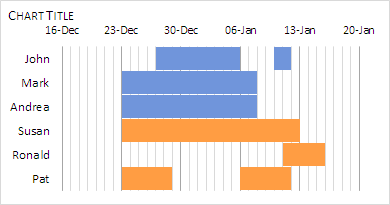
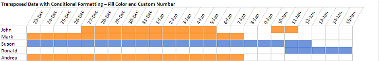
I've been going round in circles trying to figure this one out. I have to show on a graph staff on leave during a certain period, including how many per team. I'm looking for a graph with staff names on the vertical axis and each date on the horizontal axis then a plot mark showing who is away on which date, with a bar graph overlayed showing how many people from each team are away on each date. I'm not sure how to present the data on a table so the graph will work but I thought something like this might work (where the team name indicates that person is away on that date). Any help appreciated!

Date	John	Mark	Susan	Ronald	Andrea
23/12/2017		Customer Service	Accounts		Customer Service
24/12/2017		Customer Service	Accounts		Customer Service
25/12/2017		Customer Service	Accounts		Customer Service
26/12/2017		Customer Service	Accounts		Customer Service
27/12/2017	Customer Service	Customer Service	Accounts		Customer Service
28/12/2017	Customer Service	Customer Service	Accounts		Customer Service
29/12/2017	Customer Service	Customer Service	Accounts		Customer Service
30/12/2017	Customer Service	Customer Service	Accounts		Customer Service
31/12/2017	Customer Service	Customer Service	Accounts		Customer Service
1/01/2018	Customer Service	Customer Service	Accounts		Customer Service
2/01/2018	Customer Service	Customer Service	Accounts		Customer Service
3/01/2018	Customer Service	Customer Service	Accounts		Customer Service
4/01/2018	Customer Service	Customer Service	Accounts		Customer Service
5/01/2018	Customer Service	Customer Service	Accounts		Customer Service
6/01/2018		Customer Service	Accounts		Customer Service
7/01/2018		Customer Service	Accounts		Customer Service
8/01/2018			Accounts
9/01/2018			Accounts
10/01/2018			Accounts
11/01/2018			Accounts	Accounts
12/01/2018			Accounts	Accounts
13/01/2018				Accounts
14/01/2018				Accounts
15/01/2018				Accounts

<colgroup><col><col span="2"><col><col><col></colgroup><tbody>
</tbody>

 

[thisoldman]

I believe you want a Gantt chart.

This is how I arranged the data (with correct years), taken from the data you showed. The numbers in columns C and D are the durations of the vacation absences in days.

Book1
	A	B	C	D
1		Start Date	Cust Serv	Accounts
2	John	27-Dec	10
3	Mark	23-Dec	16
4	Susan	23-Dec		21
5	Ronald	11-Jan		5
6	Andrea	23-Dec	16
Sheet1

Select A1:D6 then on the Insert tab, choose "Stacked Bar".

The vertical axis was formatted with "Categories in reverse order".

The horizontal axis was formatted to Bounds – Minimum = 43085; Units – Major = 7, Minor =1.
Minor gridlines were added.

Series 1 was reformatted to have no fill and no line. Gap width for the bars was set to 5%.

The invisible series was removed from the legend.

 

[VirtualInsanity]

That looks great, only thing is it seems to only work for one block of holidays. Some people are taking two blocks of holidays e.g. John is also away on the 10th and 11th Jan. I don't really want to have to put his name on the graph twice. Do you have any suggestions on how to tweak your example to fit that?

 

[thisoldman]

It can be done as a chart but it's not as simple as my previous example. I arranged the input data like this:

Book1
	A	B	C	D	E	F
1
2	Name	Department	Start1	Return1	Start2	Return2
3	John	Customer Service	27-Dec	06-Jan	10-Jan	12-Jan
4	Mark	Customer Service	23-Dec	08-Jan
5	Andrea	Customer Service	23-Dec	08-Jan
6	Susan	Accounts	23-Dec	13-Jan
7	Ronald	Accounts	11-Jan	16-Jan
8	Pat	Accounts	23-Dec	29-Dec	06-Jan	12-Jan
StackedBar

The data I charted became this:

Book1
	H	I	J	K	L	M	N	O	P	Q
1			Customer Service				Accounts
2		Calendar Start	Start1	Duration1	Start2	Duration2	Start1	Duration1	Start2	Duration2
3	John	16-Dec	11	10	4	2	0	0	0	0
4	Mark	16-Dec	7	16	0	0	0	0	0	0
5	Andrea	16-Dec	7	16	0	0	0	0	0	0
6	Susan	16-Dec	0	0	0	0	7	21	0	0
7	Ronald	16-Dec	0	0	0	0	26	5	0	0
8	Pat	16-Dec	0	0	0	0	7	6	8	6
StackedBar

Cell Formulas
Range	Formula
J3	=IF($B3=$J$1, C3-I3, 0)
K3	=IF($B3=$J$1, D3-C3, 0)
L3	=IF(AND(E3<>"", $B3=$J$1), E3-D3, 0)
M3	=IF(AND(F3<>"", $B3=$J$1), F3-E3, 0)
N3	=IF($B3=$N$1, C3-I3, 0)
O3	=IF($B3=$N$1, D3-C3, 0)
P3	=IF(AND(E3<>"", $B3=$N$1), E3-D3, 0)
Q3	=IF(AND(F3<>"", $B3=$N$1), F3-E3, 0)

I will suggest copying your original data as you have it set up in your first post, and Paste Special – Transpose, then use conditional formatting to create an in-cells type of chart.

When a cell contains "Customer Service", it is given an orange fill. Blue cells are those that contain "Accounts". Text is hidden in those cells by using a custom number format.

;;;

That's three semicolons with no spaces.

My workbook may be downloaded from https://www.dropbox.com/s/qtoxgx4e4xvjeec/gantt_for_VirtualInsanity.xlsx?dl=0

 

[VirtualInsanity]

Thanks so, so much! That worked perfectly - and was so amazing of you to give me the workbook as a download. You really made it so easy, as I was rushing to get that finished for a meeting tomorrow and it would have taken me a long time to nut it all out on my own from the description. Really appreciate your help. Thanks again.

 

[thisoldman]

I'm happy to have helped. Thanks for getting back to us.