Greater than equal to Less than with time format formula

[waqasgul]

Hello, I'm trying to create a formula to automatically calculate on the amount of time.

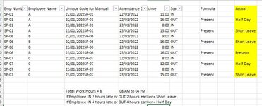
Here's the time I need to input.

trying this but not working as per my required. =IF(F4="IN","",LOOKUP((E4-E3)*24,{0,2,4},{"Short Leave","Half Day","Present"}))

If the difference between IN and OUT time is greater than or equal to 2 Hours but less than 8 hours = "Short Leave", If the difference is greater than or equal to 4 Hours but less than 8 Hours = "Half Day"

Hopefully this isn't too complex to write, thanks in advance!

 

[kevin9999]

You'll need to get the Logic right first. If, for example, the time difference was 5 hours - it would be True for both conditions:

5 hours is "greater than or equal to 2 Hours but less than 8 hours"

5 hours is "greater than or equal to 4 Hours but less than 8 Hours"

 

[kevin9999]

Try this in cell J5: =IF(H5="Present",IF((G5-G4)*24>=8,"Present",IF((G5-G4)*24>=4,"Half Day","Short Leave")))

 

[shknbk2]

Another possible solution:

=IF(F4="IN","",LOOKUP((E4-E3)*24,{4,6,8},{"Half Day","Short Leave","Present"}))

 

[kevin9999]

Try this in cell J5: =IF(H5="Present",IF((G5-G4)*24>=8,"Present",IF((G5-G4)*24>=4,"Half Day","Short Leave")))

Sorry, should have read

=IF(H5="Present",IF((E5-E4)*24>=8,"Present",IF((E5-E4)*24>=4,"Half Day","Short Leave")))

 

[waqasgul]

Great help both of you, outstanding and Thank you So much for your precious help.

@kevin9999 can you please help once more. how do i change in the formula if the total duty hours are 9. and other will be same, if 2 hour late IN or earlier OUT will be mark Short Leave and 4 hour late IN or 4 hour earlier OUT will be mark Half Day.

Thank You so much.

 

[waqasgul]

Another possible solution:

=IF(F4="IN","",LOOKUP((E4-E3)*24,{4,6,8},{"Half Day","Short Leave","Present"}))

@shknbk2 in this how can i change as per below. is this possible please?

can you please help once more. how do i change in the formula if the total duty hours are 9. and other will be same, if 2 hour late IN or earlier OUT will be mark Short Leave and 4 hour late IN or 4 hour earlier OUT will be mark Half Day.

 

[kevin9999]

Great help both of you, outstanding and Thank you So much for your precious help.

@kevin9999 can you please help once more. how do i change in the formula if the total duty hours are 9. and other will be same, if 2 hour late IN or earlier OUT will be mark Short Leave and 4 hour late IN or 4 hour earlier OUT will be mark Half Day.

Thank You so much.

Try this to start

=IF(H5="Present",IF((E5-E4)*24>=9,"Present",IF((E5-E4)*24>=4,"Half Day","Short Leave")))

 

[shknbk2]

Well, for mine, it would be simple to change it to this for the 9-hour days:

=IF(F4="IN","",LOOKUP((E4-E3)*24,{4,7,9},{"Half Day","Short Leave","Present"}))

But I wanted to find a formula that wouldn't have to be manually changed. I haven't found that the "7" and "9" values in the array can be cell references. Therefore, rather than using LOOKUP, I searched for another solution.

This one below works based on the cell with "Total Work Hours = 8". The ISNUMBER/SEARCH function returns 1 if the cell contains "9" and returns 0 otherwise. If the total work hours is 8, nothing is subtracted from the time difference (e.g., 8 hours in the fourth day - 8am to 4pm), so the result is "Present". However, if the work day was 9 hours, 1 hour is subtracted so the result is 7 hours, which means that that day is "Short Leave" since the employee left at 4pm rather than 5pm. In the formula, $C$17 is the total work hours cell. Change it if yours ends up being different.

I also changed the {4,6,8} to {0,6,8} since the 4-hour day for SP-07 results in "#N/A" for missing 5 hours in a 9-hour day; however, you can change it back to 4 if you prefer. If you want some other code to indicate working less than 4 hours, you can add another term at the beginning of the "Half Day" array for the 0-4 hour range, for example, and make the first array {0,4,6,8}.

=IF(F4="IN","",LOOKUP((E4-E3)*24-(--ISNUMBER(SEARCH("9",$C$17))),{0,6,8},{"Half Day","Short Leave","Present"}))

 

[waqasgul]

@shknbk2 you did inspirational help, bundle of thanks for your great help.