Handicap auto stablefood formula

[brynlee147]

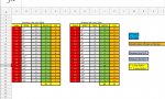
I've created a spreadsheet that has a gold course holes 1-18 each with their stroke index, also got coloums with amount of shots taken and points, I've managed to get the points and shots to add up automatically at the end, but put these in manually one by one, what I would like is for example if a golfer is a 22 handicap and he plays a hole which is index 2, he will get 2 shots extra on that and when I type the shots taken in, I would like it to automatically calculate the points awarded etc.. Same for an 18 handicap who would get 1 shot on every hole, anything under 18 then involes no shots etc

 

[Snakehips]

@brynlee147
Cannot see your image but here is an example of how you can approach this.

Book1
	B	C	D	E	F	G	H
1
2	Player	Fred	H/Cap	22
3			Hole	Par	SI	Gross	Points
4			1	4	9	4	3
5			2	3	17	3	3
6			3	4	13	5	2
7			4	4	1	4	4
8			5	4	5	6	1
9			6	3	15	4	2
10			7	5	7	7	1
11			8	4	3	5	3
12			9	4	11	3	4
13			Out	35		38	19
14			10	3	18	4	2
15			11	4	12	4	3
16			12	5	2	6	3
17			13	4	8	3	4
18			14	3	14	5	1
19			15	5	4	5	4
20			16	3	16	5	1
21			17	5	6	4	4
22			18	5	10	6	2
23			In	37		42	24
24			Out	35		38	19
25			Total	72		80	43
Sheet1

Cell Formulas
Range	Formula
G13, H13	G13	=SUM(G4:G11)
H4:H12, H14:H21	H4	=IF(G4-($E$2>=F4)-($E$2-18)>=F4<1,0,E4-L4+2)
H22	H22	=IF(G22-($E$2>=F22)+(($E$2-18)>=F22)<1,0,E22-L22+2)
G23:H23	G23	=SUM(G14:G22)
G24:H24	G24	=G13
G25:H25	G25	=SUM(G23:G24)

Hope that helps.

 

[brynlee147]

@brynlee147
Cannot see your image but here is an example of how you can approach this.

Book1
	B	C	D	E	F	G	H
1
2	Player	Fred	H/Cap	22
3			Hole	Par	SI	Gross	Points
4			1	4	9	4	3
5			2	3	17	3	3
6			3	4	13	5	2
7			4	4	1	4	4
8			5	4	5	6	1
9			6	3	15	4	2
10			7	5	7	7	1
11			8	4	3	5	3
12			9	4	11	3	4
13			Out	35		38	19
14			10	3	18	4	2
15			11	4	12	4	3
16			12	5	2	6	3
17			13	4	8	3	4
18			14	3	14	5	1
19			15	5	4	5	4
20			16	3	16	5	1
21			17	5	6	4	4
22			18	5	10	6	2
23			In	37		42	24
24			Out	35		38	19
25			Total	72		80	43
Sheet1

Cell Formulas
Range	Formula
G13, H13	G13	=SUM(G4:G11)
H4:H12, H14:H21	H4	=IF(G4-($E$2>=F4)-($E$2-18)>=F4<1,0,E4-L4+2)
H22	H22	=IF(G22-($E$2>=F22)+(($E$2-18)>=F22)<1,0,E22-L22+2)
G23:H23	G23	=SUM(G14:G22)
G24:H24	G24	=G13
G25:H25	G25	=SUM(G23:G24)

Hope that helps.

Thankyou for your advice and help, I shall try this later today when I get to sit down, really appreciate your williness to help. I've attached my orginal start of it before your help, it was work in progress and a shout for help lol... I'm a novice with excel formulas
Regards
Bryn

 

[jimrward]

@Snakehips your formulas reference column L but not shown in graphic also I would add in $E$2-36 into the scenario for larger handicaps
i have a similar spreadsheet from many years ago but can’t locate it at the moment but it’s on the same lines as what you have suggested

 

[Snakehips]

@jimrward Thanks. I had just spotted that myself and will correct and re-post shortly.
I must have picked up off a test column and not edited appropriately.
I'm not hung over, so it must be an age thing!!

 

[brynlee147]

@brynlee147
Cannot see your image but here is an example of how you can approach this.

Book1
	B	C	D	E	F	G	H
1
2	Player	Fred	H/Cap	22
3			Hole	Par	SI	Gross	Points
4			1	4	9	4	3
5			2	3	17	3	3
6			3	4	13	5	2
7			4	4	1	4	4
8			5	4	5	6	1
9			6	3	15	4	2
10			7	5	7	7	1
11			8	4	3	5	3
12			9	4	11	3	4
13			Out	35		38	19
14			10	3	18	4	2
15			11	4	12	4	3
16			12	5	2	6	3
17			13	4	8	3	4
18			14	3	14	5	1
19			15	5	4	5	4
20			16	3	16	5	1
21			17	5	6	4	4
22			18	5	10	6	2
23			In	37		42	24
24			Out	35		38	19
25			Total	72		80	43
Sheet1

Cell Formulas
Range	Formula
G13, H13	G13	=SUM(G4:G11)
H4:H12, H14:H21	H4	=IF(G4-($E$2>=F4)-($E$2-18)>=F4<1,0,E4-L4+2)
H22	H22	=IF(G22-($E$2>=F22)+(($E$2-18)>=F22)<1,0,E22-L22+2)
G23:H23	G23	=SUM(G14:G22)
G24:H24	G24	=G13
G25:H25	G25	=SUM(G23:G24)

Hope that helps.

Thankyou for your advice and help, I shall try this later today when I get to sit down, really appreciate your williness to help. I've attached my orginal start of it before your help, it was work in progress and a shout for help lol... I'm a novice with excel for
Regards
Bryn

@jimrward Thanks. I had just spotted that myself and will correct and re-post shortly.
I must have picked up off a test column and not edited appropriately.
I'm not hung over, so it must be an age thing!!

Thanks guys...... I can defo relate to an age thing on some things lol

 

[brynlee147]

Thankyou for your advice and help, I shall try this later today when I get to sit down, really appreciate your williness to help. I've attached my orginal start of it before your help, it was work in progress and a shout for help lol... I'm a novice with excel for
Regards
Bryn

Thanks guys...... I can defo relate to an age thing on some things lol

I would like it cover from 0 handicap to 36 as I will use it against various players with various handicaps..

 

[Snakehips]

Sorry for the delay.

Try this.....

Book1
	A	B	C	D	E
1
2		Player			Hcap
3		Brynlee			21.5
4	Index	Hole	Par	Gross	Points
5	11	1	3	5	1
6	1	2	5	7	2
7	7	3	4	4	3
8	5	4	4	8	0
9	15	5	3	5	1
10	13	6	5	7	1
11	3	7	3	5	2
12	17	8	4	5	2
13	9	9	5	4	4
14	2	10	5	9	0
15	14	11	4	6	1
16	18	12	3	4	2
17	4	13	3	6	1
18	12	14	3	5	1
19	6	15	4	5	2
20	10	16	4	6	1
21	16	17	4	4	3
22	8	18	3	4	2
23				99	29
Sheet1 (2)

Cell Formulas
Range	Formula
E5:E22	E5	=IF(D5<1,0,MAX(C5-(D5-((ROUND($E$3,)>=A5)+((ROUND($E$3,)-18)>=A5)))+2,0))
D23:E23	D23	=SUM(D5:D22)

 

[brynlee147]

Sorry for the delay.

Try this.....

Book1
	A	B	C	D	E
1
2		Player			Hcap
3		Brynlee			21.5
4	Index	Hole	Par	Gross	Points
5	11	1	3	5	1
6	1	2	5	7	2
7	7	3	4	4	3
8	5	4	4	8	0
9	15	5	3	5	1
10	13	6	5	7	1
11	3	7	3	5	2
12	17	8	4	5	2
13	9	9	5	4	4
14	2	10	5	9	0
15	14	11	4	6	1
16	18	12	3	4	2
17	4	13	3	6	1
18	12	14	3	5	1
19	6	15	4	5	2
20	10	16	4	6	1
21	16	17	4	4	3
22	8	18	3	4	2
23				99	29
Sheet1 (2)

Cell Formulas
Range	Formula
E5:E22	E5	=IF(D5<1,0,MAX(C5-(D5-((ROUND($E$3,)>=A5)+((ROUND($E$3,)-18)>=A5)))+2,0))
D23:E23	D23	=SUM(D5:D22)

Hi, once again thankyou, there is no need for apology, as I mentioned I'm a novice with excel formulas, so just trying to learn... I will try what you have sent with Great appreciation. Would what you done work for any handicap, or is there a aspect I would need to change for what ever the handicap may be, because mine could change from 22 to let's just say 16 for example..
Much apprection
Kind regards
Bryn
Sorry to ask so much, but it's only for me to try and understand and learn G5

 

[Snakehips]

Bryn, you are most welcome.

If you change the handicap value entered in cell E3, the points scored will change accordingly.

Below, I have made a small formula change( E$3 rather than $E$3) Thus I was able to copy A2:E23 and paste it to G2:K23 to give a second scorecard for your opponent.

NB: Click the BB2XL Copy icon, just above the 2 in my response table and you should then be able to paste it all into your spreadsheet.

Book1
	A	B	C	D	E	F	G	H	I	J	K
2		Player			Hcap			Player			Hcap
3		Brynlee			21.5			Shakey			16
4	Index	Hole	Par	Gross	Points		Index	Hole	Par	Gross	Points
5	11	1	3	5	1		11	1	3	6	0
6	1	2	5	7	2		1	2	5	7	1
7	7	3	4	4	3		7	3	4	5	2
8	5	4	4	8	0		5	4	4	5	2
9	15	5	3	5	1		15	5	3	4	2
10	13	6	5	7	1		13	6	5	4	4
11	3	7	3	5	2		3	7	3	3	3
12	17	8	4	5	2		17	8	4	4	2
13	9	9	5	4	4		9	9	5	6	2
14	2	10	5	9	0		2	10	5	7	1
15	14	11	4	6	1		14	11	4	6	1
16	18	12	3	4	2		18	12	3	4	1
17	4	13	3	6	1		4	13	3	10	0
18	12	14	3	5	1		12	14	3	3	3
19	6	15	4	5	2		6	15	4	4	3
20	10	16	4	6	1		10	16	4	6	1
21	16	17	4	4	3		16	17	4	4	3
22	8	18	3	4	2		8	18	3	4	2
23				99	29					92	33
Sheet1 (2)

Cell Formulas
Range	Formula
E5:E22, K5:K22	E5	=IF(D5<1,0,MAX(C5-(D5-((ROUND(E$3,)>=A5)+((ROUND(E$3,)-18)>=A5)))+2,0))
D23:E23, J23:K23	D23	=SUM(D5:D22)