Handicap Score Differentials up to 20 scores

andycap

New Member
Joined
Feb 24, 2021
Messages
15
Office Version
  1. 365
Platform
  1. Windows
Hello,

I have a very nice and detailed Excel database I use for our golf league. In case a golfer sees this, we use the Stableford "points" system rather than "strokes".

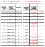
Up until now we have kept our averaging simple by only averaging the best 8 scores out of 20. For golfers with less than 8 scores then those scores were used for the average and then the Best 8 kicked in after the 9th round. Now we have to align with the 2020 USGA Handicap Index and therefore there will be different averages and adjustments based on the number of rounds. I've attached an image that showing a chart. The LEFT side of the chart is the USGA chart and then I added the RIGHT side and converted it to points using our points system for our requirements. FYI, this forum provided me the below formula and rule for conditional formatting and that's why I'm back here! :) Thanks, @Fluff

Currently this is the formula used for averaging the Best 8 out of 20 scores:
=IFERROR(AVERAGE(LARGE($H69:$AA69,SEQUENCE(MIN(8,COUNTIFS($H69:$AA69,">0"))))),0)

I also use Conditional Formatting to highlight the Best 8 scores that are used for the average.
=RANK(H69,$H69:$AA69)+COUNTIFS($H69:H69,H69)-1<=8
Going forward I would need this to adjust as the number of rounds increases and which scores are being used for averaging and, if possible, a way of showing the adjustment.

Looking at the RIGHT side of the chart you can see that for rounds 2 thru 20 there is specific averaging and adjustments after each round. The first round is fixed and doesn't need to be part of the formula. I have no idea how to go about writing a formula to address 20 different averages and adjustments.

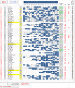
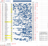
The other image is of the sheet used for what we call our "Quotas".

Is this possible?

Thank you,
Andy
 

Attachments

  • usga first 20 scores.png
    usga first 20 scores.png
    34.2 KB · Views: 90
  • Sunday, Quotas, Aug 8, 2021.png
    Sunday, Quotas, Aug 8, 2021.png
    203.4 KB · Views: 93

Excel Facts

Do you hate GETPIVOTDATA?
Prevent GETPIVOTDATA. Select inside a PivotTable. In the Analyze tab of the ribbon, open the dropown next to Options and turn it off
Something like this:

Book1
GHIJKLMNOPQRSTUVWXYZAAABACADAEAFAGAH
1
2ScoreAdjustment# of scores# to includeAdjustment
3313336353338413736293429343930333636333537.3750102
423263331331212
518 2411
62223232510
7232425252621
826272829291720
93131313232320930
102728293031353311240
1112354676.501550
12  1760
1325252728313339323601970
1421233025262930272829322330.2502080
15  
16
Sheet2
Cell Formulas
RangeFormula
AC3:AC15AC3=IFERROR(AVERAGE(LARGE(H3:AA3,SEQUENCE(VLOOKUP(COUNT(H3:AA3),AF$3:AH$14,2)))),"")
AD3:AD15AD3=IFERROR(VLOOKUP(COUNT(H3:AA3),AF$3:AH$14,3),"")
Cells with Conditional Formatting
CellConditionCell FormatStop If True
H3:AA15Expression=H3>=LARGE($H3:$AA3,VLOOKUP(COUNT($H3:$AA3),$AF$3:$AH$14,2))textNO


I originally had the table embedded within the formulas, but you can't do that for Conditional Formatting formulas, so I put it into a range (AF3:AH14) which you can put anywhere. I wasn't quite sure what to do with a single score (row 5), so it prints nothing. The other issue is with the Conditional Formatting rule. It checks to see if the value is >= to the nth highest score, but in case of ties, it will highlight more than n. Row 14 has 12 scores, so it should include 4 scores, but the 4th highest is 29, which appears twice, so both are highlighted. There might be a way to fix that, but the score in AC only includes the right amount.

Hope this helps!
 
Upvote 0
Horrible CF formula, but it does address the problem of highlighting duplicate scores:

Book1
HIJKLMNOPQRSTUVWXYZAAABACADAEAFAGAH
1
2ScoreAdjustment# of scores# to includeAdjustment
3313336353338413736293629343930333636333537.3750102
423263331331212
518 2411
62223232510
7232425252621
826272829291720
93131313232320930
102728293031353311240
1112354676.501550
12  1760
1325252728313339323601970
1421233025262930272829322330.2502080
15  
Sheet2
Cell Formulas
RangeFormula
AC3:AC15AC3=IFERROR(AVERAGE(LARGE(H3:AA3,SEQUENCE(VLOOKUP(COUNT(H3:AA3),AF$3:AH$14,2)))),"")
AD3:AD15AD3=IFERROR(VLOOKUP(COUNT(H3:AA3),AF$3:AH$14,3),"")
Cells with Conditional Formatting
CellConditionCell FormatStop If True
H3:AA15Expression=OR(H3>LARGE($H3:$AA3,VLOOKUP(COUNT($H3:$AA3),$AF$3:$AH$14,2)),AND(H3=LARGE($H3:$AA3,VLOOKUP(COUNT($H3:$AA3),$AF$3:$AH$14,2)),COUNTIF($H3:H3,H3)<=VLOOKUP(COUNT($H3:$AA3),$AF$3:$AH$14,2)-COUNTIF($H3:$AA3,">"&LARGE($H3:$AA3,VLOOKUP(COUNT($H3:$AA3),$AF$3:$AH$14,2)))))textNO
 
Upvote 0
Hey Eric,

Man, you rock! It looks great so far with one exception....it's not adding the "Adjustment" to the Quota. See attached image. I'm using Row 69 with Player "Test 1". I added column "C" as the "Adjustment" column but it's not adding the adjustment to the Quota (column B). I've went through all 20 scores and the formula seems to be working great and so is CF. The only exception is what I mentioned about it adding the Adjustment to the Quota.

You probably noticed that cells AG56:AI67 is the reference range.

Andy
 

Attachments

  • freq-usga-test.png
    freq-usga-test.png
    209.4 KB · Views: 18
Upvote 0
I wasn't sure how to handle the adjustment, which is why I put it in a separate column. You can simply add those 2 columns, or combine the formulas like this:

Excel Formula:
=IFERROR(AVERAGE(LARGE(H3:AA3,SEQUENCE(VLOOKUP(COUNT(H3:AA3),AF$3:AH$14,2))))+VLOOKUP(COUNT(H3:AA3),AF$3:AH$14,3),"")

Awesome! I think it's all working now! One more question....I have to do CF on 70 Rows. Is there a way of doing them as a whole or do I have to do one-by-one???
 
Upvote 0
Oh my! You DEFINITELY don't want to do them one-by-one! Especially with a monster formula like that! Just select the entire range you want to put the CF in, H3:AA72 I assume. Then click Conditional Formatting > New Rule > Use a formula, and paste the formula in. Make sure to change the address of the lookup table to match where you have it. Make sure the rest of the addresses refer to the top row of your range, and that the left and right columns are identified properly and with the $ in front. (The formula box is quite small and hard to work with - I often work on the formula in Notepad, then paste the final result in the formula box.) Conditional Formatting formulas work like formulas on the worksheet. If you drag a formula on the worksheet, the addresses are changed to reflect the new relative position, and the same thing is true for CF formulas within the range you selected.

Glad this works for you!
 
Upvote 0
Eric, I have similar question.

Except my league uses the lowest scores to calculate an index.

I am trying to get the CF to not highlight multiples of the same number if they are the lowest. If the lowest score is 35 and I have 3 of them, but only want to highlight two of them. I am also having a hard time getting the CF to translate to the next person.

Any help is appreciated.

WHS Handicaps.xlsx
ABCDGHIJKLMNOPQRSTUVWXYZAA
1Combined Men's League's ScoresMost Recent "Adjusted Gross Scores" Provided from Golf Genius
2Handle 18 hole IndexRound CountScores UsedAverage Score1234567891011121314151617181920
3Golfer 1-4.05234.003337353635
4Golfer 216.21140.0040
5
6
7
8
9
10
11
12
13
14
15
16
17
18
19
20
21
22
23
24
25
26
27
28
Master
Cell Formulas
RangeFormula
B3:B4B3=IFS(C3=1,((113/61)*(G3-34.55)-2),C3=2,((113/61)*(G3-34.55)-2),C3=3,((113/61)*(G3-34.55)-2),C3=4,((113/61)*(G3-34.55)-1),C3=5,((113/61)*(G3-34.55)-1),C3=6,((113/61)*(G3-34.55)-1),C3>=6,((113/61)*(G3-34.55)))*2
C3:C4C3=COUNT(H3:AA3)
D3:D4D3=IF(ISNA(INDEX($E$3:$F$22,MATCH(C3,$E$3:$E$22,0),2,FALSE)),0,(INDEX($E$3:$F$22,MATCH(C3,$E$3:$E$22,0),2)))
G3:G4G3=IFS(C3=1,(AVERAGE(SMALL(H3:NPX3,{1}))),C3=2,AVERAGE(SMALL(H3:NPX3,{1})),C3=3,AVERAGE(SMALL(H3:NPX3,{1,2})),C3=4,AVERAGE(SMALL(H3:NPX3,{1,2})),C3=5,AVERAGE(SMALL(H3:NPX3,{1,2})),C3=6,AVERAGE(SMALL(H3:NPX3,{1,2})),C3=7,AVERAGE(SMALL(H3:NPX3,{1,2})),C3=8,AVERAGE(SMALL(H3:NPX3,{1,2})),C3=9,AVERAGE(SMALL(H3:NPX3,{1,2,3})),C3=10,AVERAGE(SMALL(H3:NPX3,{1,2,3})),C3=11,AVERAGE(SMALL(H3:NPX3,{1,2,3})),C3=12,AVERAGE(SMALL(H3:NPX3,{1,2,3,4})),C3=13,AVERAGE(SMALL(H3:NPX3,{1,2,3,4})),C3=13,AVERAGE(SMALL(H3:NPX3,{1,2,3,4})),C3=14,AVERAGE(SMALL(H3:NPX3,{1,2,3,4})),C3=15,AVERAGE(SMALL(H3:NPX3,{1,2,3,4,5})),C3=16,AVERAGE(SMALL(H3:NPX3,{1,2,3,4,5})),C3=17,AVERAGE(SMALL(H3:NPX3,{1,2,3,4,5,6})),C3=18,AVERAGE(SMALL(H3:NPX3,{1,2,3,4,5,6})),C3=19,AVERAGE(SMALL(H3:NPX3,{1,2,3,4,5,6,7})),C3>=20,AVERAGE(SMALL(H3:NPX3,{1,2,3,4,5,6,7,8})))
Cells with Conditional Formatting
CellConditionCell FormatStop If True
H3:AA150Cellcontains a blank value textYES
H3:AA150Expression=H3<=SMALL($H$3:$AA$3, $D$3)textNO
 
Upvote 0
@Eric W I see you helped out, I hope you get a chance to have a look for me. Maybe help with simpler formulas?
 
Upvote 0
Welcome to MrExcel!

For future reference, it's probably best to open a new thread, so that more people will see it. You can certainly reference the earlier thread, or even tag the helper (as you did in your second message).

But given that, try this:

Book1
ABCDGHIJKLMNOPQRSTUVWXYZAA
1Combined Men's League's ScoresMost Recent "Adjusted Gross Scores" Provided from Golf Genius
2Handle 18 hole IndexRound CountScores UsedAverage Score1234567891011121314151617181920
3Golfer 1-4.05234.003337353635
4Golfer 216.21140.0040
Sheet1
Cell Formulas
RangeFormula
B3:B4B3=2*(113/61)*(G3-34.55)-LOOKUP(C3,{1,4,7},{4,2,0})
C3:C4C3=COUNT(H3:AA3)
D3:D4D3=MATCH(C3,{1,3,9,12,15,17,19,20})
G3:G4G3=AVERAGE(SMALL(H3:NPX3,SEQUENCE(D3)))
Cells with Conditional Formatting
CellConditionCell FormatStop If True
H3:AA4Expression=LET(s,SMALL($H3:$AA3,$D3),AND(H3<>"",OR(H3<s,AND(H3=s,COUNTIF($H3:H3,s)<=$D3-COUNTIF($H3:$AA3,"<"&s)))))textNO


I did simplify some of the formulas, and I used some of the new functionality in Excel 365 to make them easier. Let me know how this works for you!
 
Upvote 0

Forum statistics

Threads
1,214,599
Messages
6,120,448
Members
448,966
Latest member
DannyC96

We've detected that you are using an adblocker.

We have a great community of people providing Excel help here, but the hosting costs are enormous. You can help keep this site running by allowing ads on MrExcel.com.
Allow Ads at MrExcel

Which adblocker are you using?

Disable AdBlock

Follow these easy steps to disable AdBlock

1)Click on the icon in the browser’s toolbar.
2)Click on the icon in the browser’s toolbar.
2)Click on the "Pause on this site" option.
Go back

Disable AdBlock Plus

Follow these easy steps to disable AdBlock Plus

1)Click on the icon in the browser’s toolbar.
2)Click on the toggle to disable it for "mrexcel.com".
Go back

Disable uBlock Origin

Follow these easy steps to disable uBlock Origin

1)Click on the icon in the browser’s toolbar.
2)Click on the "Power" button.
3)Click on the "Refresh" button.
Go back

Disable uBlock

Follow these easy steps to disable uBlock

1)Click on the icon in the browser’s toolbar.
2)Click on the "Power" button.
3)Click on the "Refresh" button.
Go back
Back
Top