Help in creating a chart

[leontin]

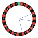
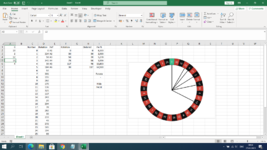
Hi, guys. I'm pretty new to excel and i'm struggling to create a basic chart like in the image.
Can anyone help me with a video\tutorial or something to create this? I guess it's not complicated to do.
I have searched on the internet buy i couldn't find something similiar. I guess it will be a combination of doughnut with pie chart?

What i want is up to six pointers\lines, eache one of them coresponding to a value in a cell.
Example: cell: A1=25, A2=6 etc and i need pointers in the circle to match the value in the cell with the number in the circle and if no value in the cell then no pointer.

Thank you in advance.

 

[Snakehips]

@leontin Welcome to the forum
I don't think you can accomplish this without using vba.
If you are happy / able to include vba then let me know and i will try and help.

 

[leontin]

@leontin Welcome to the forum
I don't think you can accomplish this without using vba.
If you are happy / able to include vba then let me know and i will try and help.

Thank you for your interest in helping me.
Yes, of course, I'm ok with VBA, my workbook is already macro-enabled, i have made some clickable buttons using VBA.

 

[Snakehips]

What I am envisaging is that you edit the circle image image to remove the pointers. I have done that using Photoshop.
Then you will insert an appropriately sized and formatted pie chart to sit in the centre of the circel.

The major issue with trying to point to the numbers is that the 'Angle of first sector rotation' will vary with each first number.
As an absolute minimum, it will need vba to detect and make change to this angle.
Other than that, I think I can use formulas and helper columns to determine the Pie chart values required to point to the 1 - 6 values in column A

Does this sound like a workable approach for you?

 

[Snakehips]

Here goes....

Assuming your number entries are in A1 : A6 and that you set up the helper columns. (helper columns may be hidden if you wish)

Copy / paste the XL2BB below.

PERSONAL.XLSB
	A	B	C	D	E	F	G	H	I	J
1			Number	Rotation	Ref	Rotation		Ordered	Pie %
2	19		0	0	A1
3			1	224	A2	30
4	5		2	58	A3			30	18.611
5	22		3	341	A4	184		97	24.167
6	6		4	39	A5	272		184	24.444
7			5	184	A6	97		272	32.778
8			6	97
9			7	301					Rotate
10			8	155					30
11			9	262
12			10	175					Hide
13			11	136					FALSE
14			12	321
15			13	117
16			14	243
17			15	20
18			16	204
19			17	78
20			18	282
21			19	30
22			20	233
23			21	49
24			22	272
25			23	165
26			24	194
27			25	68
28			26	351
29			27	107
30			28	311
31			29	292
32			30	146
33			31	253
34			32	10
35			33	214
36			34	88
37			35	331
38			36	127
Sheet3

Cell Formulas
Range	Formula
H2:H7	H2	=IFERROR(LARGE($F$2:$F$7,ROWS(H1:H$6)),"")
I2:I6	I2	=IF(H2="","",(H3-H2)/3.6)
I7	I7	=IF(H7="","",(100-SUM(I2:I6)))
F2:F7	F2	=IF(A1="","",INDEX($D$2:$D$38,MATCH(A1,$C$2:$C$38,0)))
I10	I10	=MIN(H2:H7)
I13	I13	=COUNTA(A1:A6)=0

Cells with Data Validation
Cell	Allow	Criteria
A1:A6	Whole number	between 0 and 36

Ideally, set Data validation for the input range A1:A6 to limit entry to Numbers 0 to 36.

Then insert a Pie chart and the edited image of your "Circle' such that the original lines have been removed.

Set the Pie chart Data Range to I2:I7 Size the Pie to fit the inner circle. Remove Legend etc.
Format to the Data Series Fill to 'No Fill" Border Colour - Black. Shadow Pre-Set is set to No Shadow etc so that the whole chart is simple black and white.
Position the image over the chart. White fill the surrounding cell range.

Copy paste the following code to the Worksheet Code Module

Private Sub Worksheet_Change(ByVal Target As Range)

If Intersect(Target, Range("A1:A6")) Is Nothing Then Exit Sub
'***** EDIT THE CHART NAME below TO SUIT ******
ActiveSheet.ChartObjects("Chart 4").Chart.Rotation = Range("I10").Value
ActiveSheet.ChartObjects("Chart 4").Visible = Not (Range("I13").Value)

End Sub

Determine your chart name and edit the code accordingly.

Then see if it works?

 

[Snakehips]

So, you need the chart over white cells and the circle over the chart.

Below is the circle without lines.

 

[leontin]

wow, it's more complex than i thought. I will try it later today and i will let you know. thank you for your help!

 

[leontin]

Here goes....

Assuming your number entries are in A1 : A6 and that you set up the helper columns. (helper columns may be hidden if you wish)

Copy / paste the XL2BB below.

PERSONAL.XLSB
	A	B	C	D	E	F	G	H	I	J
1			Number	Rotation	Ref	Rotation		Ordered	Pie %
2	19		0	0	A1
3			1	224	A2	30
4	5		2	58	A3			30	18.611
5	22		3	341	A4	184		97	24.167
6	6		4	39	A5	272		184	24.444
7			5	184	A6	97		272	32.778
8			6	97
9			7	301					Rotate
10			8	155					30
11			9	262
12			10	175					Hide
13			11	136					FALSE
14			12	321
15			13	117
16			14	243
17			15	20
18			16	204
19			17	78
20			18	282
21			19	30
22			20	233
23			21	49
24			22	272
25			23	165
26			24	194
27			25	68
28			26	351
29			27	107
30			28	311
31			29	292
32			30	146
33			31	253
34			32	10
35			33	214
36			34	88
37			35	331
38			36	127
Sheet3

Cell Formulas
Range	Formula
H2:H7	H2	=IFERROR(LARGE($F$2:$F$7,ROWS(H1:H$6)),"")
I2:I6	I2	=IF(H2="","",(H3-H2)/3.6)
I7	I7	=IF(H7="","",(100-SUM(I2:I6)))
F2:F7	F2	=IF(A1="","",INDEX($D$2:$D$38,MATCH(A1,$C$2:$C$38,0)))
I10	I10	=MIN(H2:H7)
I13	I13	=COUNTA(A1:A6)=0

Cells with Data Validation
Cell	Allow	Criteria
A1:A6	Whole number	between 0 and 36

Ideally, set Data validation for the input range A1:A6 to limit entry to Numbers 0 to 36.

Then insert a Pie chart and the edited image of your "Circle' such that the original lines have been removed.

View attachment 37437

Set the Pie chart Data Range to I2:I7 Size the Pie to fit the inner circle. Remove Legend etc.
Format to the Data Series Fill to 'No Fill" Border Colour - Black. Shadow Pre-Set is set to No Shadow etc so that the whole chart is simple black and white.
Position the image over the chart. White fill the surrounding cell range.

Copy paste the following code to the Worksheet Code Module

Private Sub Worksheet_Change(ByVal Target As Range)

If Intersect(Target, Range("A1:A6")) Is Nothing Then Exit Sub
'***** EDIT THE CHART NAME below TO SUIT ******
ActiveSheet.ChartObjects("Chart 4").Chart.Rotation = Range("I10").Value
ActiveSheet.ChartObjects("Chart 4").Visible = Not (Range("I13").Value)

End Sub

Determine your chart name and edit the code accordingly.

Then see if it works?

I have tested right now and works like a charm! Exactly what I wanted. Thank You so much!

 

[Snakehips]

Good to hear and, you are most welcome. It was an interesting little puzzle to crack.

 

[leontin]

Good to hear and, you are most welcome. It was an interesting little puzzle to crack.

Hi, Snakehips. I have discovered a problem. I have applied the code to my main worksheet and apparently it's not working because the A1:A6 cells for the input of the numbers contains a formula.
Pointers indicating diferent numbers or none at all... How can i workaround this? Waiting for your reply. Thanks.