Hi,
I’ve written a code for a workbook, and would like to make it more dynamic but not sure how to do that. I’ve tried a few times with INDEX and MATCH but still quite new to excel so I haven’t had any success. Basically what I want to do is from the "Scoring 4" sheet, I want to get the quartile rank associated with a specific company and metric. The underlying data is in the "data" sheet, and the calculations for quartiles are in the "quartiles" sheet. My biggest concern is the first part of the equation so just matching the metric on the first row with the value on the "data" sheet. the second part which matches the D-column with the the "quartiles" sheet I think is less of an issue but thankful for any help there as well.
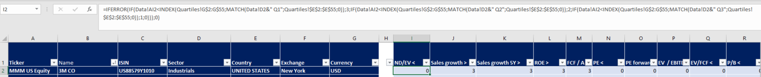
Does anyone have any idea how I can fix my issue? I’ve attatched a picture showing the code currently and I’ll write it below as well.
=IFERROR(IF(Data!AI2<INDEX(Quartiles!G$2:G$55;MATCH(Data!D2&" Q1";Quartiles!$E$2:$E$55;0));3;IF(Data!AI2<INDEX(Quartiles!G$2:G$55;MATCH(Data!D2&" Q2";Quartiles!$E$2:$E$55;0));2;IF(Data!AI2<INDEX(Quartiles!G$2:G$55;MATCH(Data!D2&" Q3";Quartiles!$E$2:$E$55;0));1;0)));0)
Thankful for any help,
Oscar
I’ve written a code for a workbook, and would like to make it more dynamic but not sure how to do that. I’ve tried a few times with INDEX and MATCH but still quite new to excel so I haven’t had any success. Basically what I want to do is from the "Scoring 4" sheet, I want to get the quartile rank associated with a specific company and metric. The underlying data is in the "data" sheet, and the calculations for quartiles are in the "quartiles" sheet. My biggest concern is the first part of the equation so just matching the metric on the first row with the value on the "data" sheet. the second part which matches the D-column with the the "quartiles" sheet I think is less of an issue but thankful for any help there as well.
Does anyone have any idea how I can fix my issue? I’ve attatched a picture showing the code currently and I’ll write it below as well.
=IFERROR(IF(Data!AI2<INDEX(Quartiles!G$2:G$55;MATCH(Data!D2&" Q1";Quartiles!$E$2:$E$55;0));3;IF(Data!AI2<INDEX(Quartiles!G$2:G$55;MATCH(Data!D2&" Q2";Quartiles!$E$2:$E$55;0));2;IF(Data!AI2<INDEX(Quartiles!G$2:G$55;MATCH(Data!D2&" Q3";Quartiles!$E$2:$E$55;0));1;0)));0)
Thankful for any help,
Oscar