Help needed with splitting data into separate columns

[yvette78]

HI everyone - i am hoping someone can help me with this excel function.

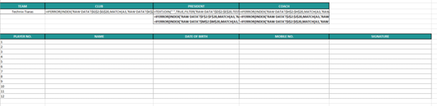
I have attached two images.....one of the data I need to split and another of the dashboard/table where i need the data to go.

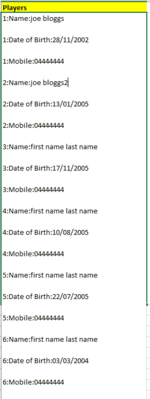
I will be receiving an excel document from a client with raw data containing many columns but what i need help with relates to the column named "PLAYERS" SO I have copied this column into a separate document to make things easier to follow. The data will be in the same format as per the attached document on sheet named RAW DATA.

The players column shows 12 players and the RAW DATA column contains each of the players NAME, DATE OF BIRTH and MOBILE NUMBER. I need to be able to extract each of these (NAME, DATA OF BIRTH and MOBILE NUMBER) into separate columns as per SHEET 2. So Player 1 on the dashboard/table, would be JOE BLOGGS (NAME COLUMN), 28/11/2002 (DATE OF BIRTH COLUMN), 04444444 (MOBILE NUMBER COLUMN).

Is there anyone that can help me? Thank you in advance.

 

[Alex Blakenburg]

I would be inclined to use Power Query but if you can rely on the player numbers being in the Raw Data, you could try something like this.

20220120 Lookup or PQ.xlsx
	A	B	C	D	E	F	G
8	PLAYER NO	NAME	DATE OF BIRTH	MOBILE NO.			Player
9	1	joe bloggs	28/11/2002	044444444			1:Name:joe bloggs
10	2	joe bloggs2	28/11/2099	099999999			1:Date of Birth:28/11/2002
11	3						1:Mobile:044444444
12	4						2:Name:joe bloggs2
13							2:Date of Birth:28/11/2099
14							2:Mobile:099999999
15
16
Sheet1

Cell Formulas
Range	Formula
B9:B10	B9	=MID(XLOOKUP($A9&":NAME:*",$G$9:$G$14,$G$9:$G$14,"Not Found",2),FIND("e:",XLOOKUP($A9&":NAME:*",$G$9:$G$14,$G$9:$G$14,"Not Found",2))+2,255)
C9:C10	C9	=MID(XLOOKUP($A9&":Date of Birth:*",$G$9:$G$14,$G$9:$G$14,"Not Found",2),FIND("h:",XLOOKUP($A9&":Date of Birth:*",$G$9:$G$14,$G$9:$G$14,"Not Found",2))+2,255)
D9:D10	D9	=MID(XLOOKUP($A9&":Mobile:*",$G$9:$G$14,$G$9:$G$14,"Not Found",2),FIND("e:",XLOOKUP($A9&":Mobile:*",$G$9:$G$14,$G$9:$G$14,"Not Found",2))+2,255)

 

[yvette78]

I would be inclined to use Power Query but if you can rely on the player numbers being in the Raw Data, you could try something like this.

20220120 Lookup or PQ.xlsx
	A	B	C	D	E	F	G
8	PLAYER NO	NAME	DATE OF BIRTH	MOBILE NO.			Player
9	1	joe bloggs	28/11/2002	044444444			1:Name:joe bloggs
10	2	joe bloggs2	28/11/2099	099999999			1:Date of Birth:28/11/2002
11	3						1:Mobile:044444444
12	4						2:Name:joe bloggs2
13							2:Date of Birth:28/11/2099
14							2:Mobile:099999999
15
16
Sheet1

Cell Formulas
Range	Formula
B9:B10	B9	=MID(XLOOKUP($A9&":NAME:*",$G$9:$G$14,$G$9:$G$14,"Not Found",2),FIND("e:",XLOOKUP($A9&":NAME:*",$G$9:$G$14,$G$9:$G$14,"Not Found",2))+2,255)
C9:C10	C9	=MID(XLOOKUP($A9&":Date of Birth:*",$G$9:$G$14,$G$9:$G$14,"Not Found",2),FIND("h:",XLOOKUP($A9&":Date of Birth:*",$G$9:$G$14,$G$9:$G$14,"Not Found",2))+2,255)
D9:D10	D9	=MID(XLOOKUP($A9&":Mobile:*",$G$9:$G$14,$G$9:$G$14,"Not Found",2),FIND("e:",XLOOKUP($A9&":Mobile:*",$G$9:$G$14,$G$9:$G$14,"Not Found",2))+2,255)

Thank you for this.....

I am still having some trouble.

These are the headings in the raw data file:-

These are the headings in the dashboard/summary (where i need to extract data to)
The TEAM column is a dropdown field and when i choose a TEAM, it then populates the CLUB, PRESIDENT & COACH.

These are the headings relating to the players.
I need it to auto-populate the players like you have done above, but when I change the TEAM, the players update according to what I have chosen.
There are 35 rows which have different teams, clubs & players.

PLAYER #

NAME

DATE OF BIRTH

MOBILE

 

[Alex Blakenburg]

You will need to provide sample data that includes the all columns to be used as criteria to extract the data you need returned.
Also if the player field does not have 1: 2: 3: etc as a prefix at the Team level (assuming that is the filter criteria), then you need to show the data as it really appears since I was relying on that to find the data.
Ideally provide the data as an Xl2BB so we can copy it into our Excel.

 

[Peter_SSs]

This is my take on it. I wasn't sure that the player numbers had to match, or if they do the players would be listed in order like the sample.

yvette78.xlsm
	K	L
1	Team Name	Players
2	Team 1	1:Name:joe bloggs
3	Team 1	1:Date of Birth:28/11/2002
4	Team 1	1:Mobile:044444444
5	Team 1	2:Name:joe bloggs2
6	Team 1	2:Date of Birth:28/11/2005
7	Team 1	2:Mobile:099999999
8	Team 2	1:Name:ken bloggs
9	Team 2	1:Date of Birth:28/11/2000
10	Team 2	1:Mobile:044444455
11	Team 2	2:Name:jon bloggs
12	Team 2	2:Date of Birth:8/1/2000
13	Team 2	2:Mobile:044449955
14	Team 2	3:Name:sam bloggs
15	Team 2	3:Date of Birth:12/4/2006
16	Team 2	3:Mobile:088444455
17
RAW DATA

yvette78.xlsm
	A	B	C	D
1	Team Name
2	Team 2
3
4
5
6	PLAYER NO	NAME	DATE OF BIRTH	MOBILE NO.
7	1	ken bloggs	28/11/2000	044444455
8	2	jon bloggs	8/1/2000	044449955
9	3	sam bloggs	12/4/2006	088444455
10	4
Dashboard

Cell Formulas
Range	Formula
B7:D10	B7	=LET(t,INDEX(FILTER('RAW DATA'!$L$2:$L$100,'RAW DATA'!$K$2:$K$100=$A$2),($A7-1)*3+COLUMNS($B:B)),IFERROR(REPLACE(t,1,FIND(":",t,5),""),""))

 

[Fluff]

Welcome to the MrExcel Message Board!

Cross-posting (posting the same question in more than one forum) is not against our rules, but the method of doing so is covered by #13 of the Forum Rules.

Be sure to follow & read the link at the end of the rule too!

Cross posted at: Help needed with splitting data into separate columns
If you have posted the question at more places, please provide links to those as well.

If you do cross-post in the future and also provide links, then there shouldn’t be a problem.

 

[yvette78]

I need some help again with regards to splitting data but this is for another document.

When a course date is chosen at A10, I want it to populate all the participants details that have the same date in the RAW DATA tab (Column G) but the data I need split comes from the PARTICIPANTS DATA CELL tab (A2).

DATA TO SPLIT: Joe Bloggs :Pizzey park:bloggs@gmail.com:0407313335:NetSetGo PARTICIPANTS NAME: JOE BLOGGS CLUB NAME: PIZZEY PARK EMAIL: bloggs@gmail.com PHONE NUMBER: 0407313335 COMPETITION:NetSetGo Please note that sometimes there may be more than one participant, so the formula will need to be able to list each participant in a separate line on the FORM. For example, L3 in the RAW DATA tab has two participants, as follows:- Joe Love :Palm Beach :bloggsf@hotmail.com:0407777777:Junior Joe Love 2 :Palm Beach :bloggs3@hotmail.com:042222222:Junior so I need Joe Love details on one line, then Joe LOVE 2's details on the next. I hope this makes sense. Thanks Document is attached

 

[yvette78]

 

[Peter_SSs]

@yvette78
It appears that you have ignored post #6 above. Please see my Conversation Message to you about that.

Cross-posted here: Split Data from one Cell into Different Columns