Help SUMIF with YTD

[shepcs]

Would greatly appreciate any help as its driving me nuts.
I'm trying to do a YTD summation given a value to lookup in a single column (Column C), then doing a ytd in the Jan-Dec columns (E:P).
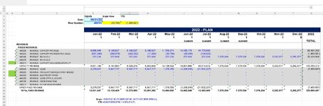
So for Inputs I have a number to lookup in a column and a date (in this case E2: 400101 and E3: 05/31/22)

For a single value its no problem, I do
=SUMIF($C:$C,E3,INDEX($E:$P,,MATCH(E2,$E$6:$P$6,0)))

And I know the YTD formula works but this is inputting a specific row (E12:P12) instead of location the row by the input number E2
=SUMIF($E$6:$P$6,"<="&E2,E12:P12)

I'm trying to combine the two and running into a problem.

Really appreciate any insight.
Thanks!!

 

[awoohaw]

How is it that you have A:A4# in your workbook? There is not an array producing expression in cell A4 (in what I copied over.) I'm not sure what range of cells that expression is meant to include?

 

[shepcs]

Thanks awoohaw. But I was trying to sum Jan-May. So 400101 should be 40,230,630

 

[shepcs]

How is it that you have A:A4# in your workbook? There is not an array producing expression in cell A4 (in what I copied over.) I'm not sure what range of cells that expression is meant to include?

I might have fat fingered that. I just changed it to A:A and still didnt work. I was trying to say search the entire column A for that Dept Partner number (That pegs the row), then by the desired YTD date (May) in this case, sum all months in columns up to and including May. Again the only inputs being a department number and YTD Date (May).

 

[awoohaw]

okay this is jan to may:

Book1
	A	B	C	D	E	F	G	H	I	J	K	L	M	N
1
2	RAW Data
3	DEPT	2022-01-31	2022-02-28	2022-03-31	2022-04-30	2022-05-31	2022-06-30	2022-07-31	2022-08-31	2022-09-30	2022-10-31	2022-11-30	2022-12-31	1905-07-14
4	400100	9866446.4	6198636.8	6198636.8	6198636.8	11768273.6	14485169.6	44778560	0	0	0	0	0	99494360
5	400101	-587340.07	-388978.11	-242392.4047	-17025.1807	-33785.4168	-55537.9333	-134921.827	0	0	0	0	0	-1459980.94
6	400160	372033.93	372033.93	372033.93	372033.93	372033.93	372033.93	372033.93	7378533.93	7378533.93	7378533.93	5292577.43	5292577.43	35324994.16
7	400170	0	0	0	0	0	0	0	0	0	0	0	0	0
8	400171	0	0	0	0	0	0	0	0	0	0	0	0	0
9
10	Reporting Page
11	Date Input	2022-05-31
12			YTD May Output
13	Dept Input	400100	#REF!	40,230,630.40
14	Dept Input	400101	#REF!	(1,269,521.18)
15	Dept Input	400160	#REF!	1,860,169.65
16	Dept Input	400170	#REF!	-
17	Dept Input	400171	#REF!	-
Sheet3

Cell Formulas
Range	Formula
C13:C17	C13	=SUM(FILTER(FILTER($B$4:$M$8,(MONTH(B$3:M$3)<=MONTH($B$11))),A:A#=B13))
D13:D17	D13	=SUMPRODUCT((--($B13=$A$4:$A$8))* (--(MONTH($B$11)>=MONTH($B$3:$N$3)))* (--(1<=MONTH($B$3:$N$3))) *($B$4:$N$8))

 

[shepcs]

Thanks Awoohaw! That totally worked. I really appreciate the help. I'll now try to figure out what its doing. I changed it to October as a test and for some reason it was including hte annual "2022" column N. Not sure why but I tweaked your formula to exclude it. Thank you again!

SUMIF HELP.xlsx
	A	B	C	D	E	F	G	H	I	J	K	L	M	N
1
2	RAW Data
3	DEPT	Jan-22	Feb-22	Mar-22	Apr-22	May-22	Jun-22	Jul-22	Aug-22	Sep-22	Oct-22	Nov-22	Dec-22	2022
4	400100	9,866,446	6,198,637	6,198,637	6,198,637	11,768,274	14,485,170	44,778,560	-	-	-	-	-	99,494,360
5	400101	(587,340)	(388,978)	(242,392)	(17,025)	(33,785)	(55,538)	(134,922)	-	-	-	-	-	(1,459,981)
6	400160	372,034	372,034	372,034	372,034	372,034	372,034	372,034	7,378,534	7,378,534	7,378,534	5,292,577	5,292,577	35,324,994
7	400170	-	-	-	-	-	-	-	-	-	-	-	-	-
8	400171	-	-	-	-	-	-	-	-	-	-	-	-	-
9
10	Reporting Page
11	Date Input	08/31/22
12			YTD May Output
13	Dept Input	400100	99,494,360
14	Dept Input	400101	(1,459,981)
15	Dept Input	400160	9,982,771
16	Dept Input	400170	-
17	Dept Input	400171	-
Sheet1 (2)

Cell Formulas
Range	Formula
C13:C17	C13	=SUMPRODUCT((--($B13=$A$4:$A$8))*(--(MONTH($B$11)>=MONTH($B$3:$M$3)))*(--(1<=MONTH($B$3:$M$3)))*($B$4:$M$8))

Cells with Conditional Formatting
Cell	Condition		Cell Format	Stop If True
B11	Expression	=#REF!<>0	text	YES
E1	Expression	=#REF!<>0	text	YES
B10:B11	Expression	=#REF!<>0	text	YES
G1:M1,C1,B10:B11,N1:N2	Expression	=#REF!<>0	text	YES

 

[awoohaw]

it is matrix math. it calculates zeros and ones to multiply by the entire data grid, if you only want 2023, then insert this somewhere in the multiplication:
(--(2023=Year($B$3:$M$3))

 

[awoohaw]

you can see how it works by highlighting each section between asterisks, press F9 to see the calculations. But, don't hit enter after that, press escape or ctrl Z to back it out.

 

[shepcs]

I will try that now. Thanks again!!

 

[awoohaw]

I will try that now. Thanks again!!

my pleasure, happy to help.

 

[Fluff]

The formula I originally supplied works, once the ranges are change to your new layout

Fluff.xlsm
	A	B	C	D	E	F	G	H	I	J	K	L	M	N
1
2	RAW Data
3	DEPT	31/01/2022	28/02/2022	31/03/2022	30/04/2022	31/05/2022	30/06/2022	31/07/2022	31/08/2022	30/09/2022	31/10/2022	30/11/2022	31/12/2022	2022
4	400100	9866446.4	6198636.8	6198636.8	6198636.8	11768273.6	14485169.6	44778560	0	0	0	0	0	99494360
5	400101	-587340.07	-388978.11	-242392.4047	-17025.18068	-33785.41683	-55537.93334	-134921.8268	0	0	0	0	0	-1459980.942
6	400160	372033.93	372033.93	372033.93	372033.93	372033.93	372033.93	372033.93	7378533.93	7378533.93	7378533.93	5292577.43	5292577.43	35324994.16
7	400170	0	0	0	0	0	0	0	0	0	0	0	0	0
8	400171	0	0	0	0	0	0	0	0	0	0	0	0	0
9
10	Reporting Page
11	Date Input	31/05/2022
12			YTD May Output
13	Dept Input	400100	40230630.4
14	Dept Input	400101	-1269521.182
15	Dept Input	400160	1860169.65
16	Dept Input	400170	0
17	Dept Input	400171	0
Main

Cell Formulas
Range	Formula
C13:C17	C13	=SUMPRODUCT(($A$4:$A$8=B13)*($B$3:$M$3<=B$11)*($B$4:$M$8))