Help with Calculating Stacked payments using banding eg tax

[MikeXYZ7]

Hi there

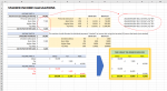
I am hoping someone can take pity on me and put me out of my misery? I have been trying to figure this out for hours! I am trying to get on top of my finances and want to make a "calculator" that can automatically work out out TAX DUE for PAYE & DIVIDENDS (both use different tax %). Hopefully this is obvious on the screen shot attached.

I have done this successfully for the first part eg assuming a £50k PAYE start, i have successfully worked out how to automatically work out the tax (please note that as i can't attach the excel file, i have shown the formula i have used in the attachment).

What i need to be able to do (and need help with) is to have a start point of £50k going into the second part (DIVIDEND section) and then allocate tax against the new income of £50k (for example) using the new tax % as shown in the figures. And it is here i just cannot work out what to do? I have tried lots of attempts but cannot get my head round how to approach this automatically (it is easy to manually do it - i have shown the answer ii am trying to achieve).

Please can someone put me out of my misery?

Best wishes

Mike

 

[MikeXYZ7]

Hi Kirk

Once again "Thank You" for helping me get this right! I've been using the solution to model a 10 year plan...and in doing so discovered an annoying error. I have however, fixed it (I think) - but wondered if you could double check?

When the Wages (Part A) figure is within £2,000 of the end of the band eg £48,500 or £148,500, this throws the dividend calculations and returns a negative number (for Tax due in dividends) - which is obviously incorrect.

What i have done to fix this is add an extra "IF" statement in cells I20, I21 & I22 that basically says "IF this cell VALUE < 0" then cell=0. If the calculation result is >0, then the VALUE is ok.

I've tested it and it works perfectly - just wanted your expert opinion on this solution?

Hope your weekend is good

Mike

 

[Dave Patton]

For your consideration.
I know you are using the other approach but I added the second table for the rates .
You can check if the tables work according to your requirements.
If you review the logic of the formulas, you can edit them for your specific requirements.
You could use Choose instead of the If functions. I deleted the example.

T202004a.xlsm
	A	B	C	D	E	F	G	H	I	J	K	L	M	N	O
1	Income
2	Regular	30,000.00	3,500.00
3	Dividends	60,000.00	14,350.00
4		90,000.00	17,850.00
5
6	Regular Income
7	Brackets	Rates	Rate Diff		Brackets	Rates	Rate Diff		Brackets	Rates	Rate Diff		Brackets	Rates	Rate Diff
8	0.00	0%	0.00%		0	0.0%	0.00%		0	0.0%	0.00%		0	0.0%	0.00%
9	12,500.00	20%	20.00%		2,000	7.5%	7.50%		2,000	32.5%	32.50%		2,000	38.1%	38.10%
10	50,000.00	40%	20.00%		20,000	32.5%	25.00%		120,000	38.1%	5.60%
11	150,000.00	45%	5.00%		120,000	38.1%	5.60%
UK

Cell Formulas
Range	Formula
C2	C2	=SUMPRODUCT(--(B2>A8:A11),B2-A8:A11,C8:C11)
C3	C3	=IF(B2<50000,SUMPRODUCT(--(B3>B_1),B3-B_1,R_1),IF(B2<150000,SUMPRODUCT(--(B3>B_2),B3-B_2,R_2),SUMPRODUCT(--(B3>B_3),B3-B_3,R_3)))
B4:C4	B4	=B2+B3
G8:G11,C8:C11,K8:K10,O8:O9	O8	=N8-N(N7)
I10	I10	=100000-MIN(B2-50000,100000)
E10	E10	=50000-MIN(B2,50000)
E11	E11	=150000-MIN(150000,B2)

Named Ranges
Name	Refers To	Cells
B_1	=UK!$E$8:$E$11	C3
B_2	=UK!$I$8:$I$10	C3
B_3	=UK!$M$8:$M$9	C3
R_1	=UK!$G$8:$G$11	C3
R_2	=UK!$K$8:$K$10	C3
R_3	=UK!$O$8:$O$9	C3

 

[KRice]

I'll look into this.

 

[KRice]

Hi Mike,
Have a look at this version. As I looked into the issue further, I encountered some other issues, and concluded that the CHOOSE(IF(ROWS=MATCH construction was overkill. I simplified that formula; and with further experimentation, I also discovered issues with the band limits. In the end, it was easier to introduce helper columns to the right (shaded with a note not to delete). Those redefine the band limits in a way that reflects how they are actually filled, starting with a 0 basis. I've tried this out with dozens of examples and found it necessary to adjust some formulas to reproduce the behavior of various online calculators. Some components of the formulas are inferred based on the observed online calculator behavior. Ideally, there would be better descriptions of detailed computation methodologies from the taxing authority, but I haven't been able to find that. The primary issue involves how to handle the allowances under certain situations. I think this version is very close to the mark. I've also added a feature that begins to phase out the personal allowance when the total income threshold is reached, at a rate of 1 pound sterling for every 2 that exceed the threshold. Please let me know if you encounter any odd results.

UKtax20200419.xlsx
	A	B	C	D	E	F	G	H	I	J	K	L	M	N	O	P	Q	R	S	T	U	V
6		Personal Allowance Phaseout Threshhold	100000
7
8		WAGES INCOME PART A							0.00	<- Taxable Inc		DO NOT DELETE
9		Total Income (Excluding Dividends)	0		Band	Rate	Start	End	TWI Allocation	Remainder		revStart	revEnd			2018-2019			2019-2020			2020-2021
10		Personal Allowance	0.00		Personal Allowance	0.000	0	12500	~~~~~	0.00					0	11850		0	12500		0	12500
11		Basic Rate	0.00		Basic Rate	0.200	12500	50000	0.00	0		0	37500		11850	46350		12500	50000		12500	50000
12		Higher Rate	0.00		Higher Rate	0.400	50000	150000	0.00	0		37500	150000		46350	150000		50000	150000		50000	150000
13		Top Rate	0.00		Top Rate	0.450	150000	1000000	0.00	0		150000	1000000		150000	1000000		150000	1000000		150000	1000000
14		TAX TO PAY IN THIS SLICE	0.00
15
16		DIVIDENDS INCOME PART B							35500	<- Taxable Div		DO NOT DELETE
17		DIVIDEND PAYMENTS	50000		Band	Rate	Start	End	TDI Allocation	Remainder		revStart	revEnd
18		Personal Allowance Carryover	12500.00		Personal Allowance C/O	0.000			~~~~~	37500.00						2018-2019			2019-2020			2020-2021
19		Dividend Allowance	2000.00		Dividend Allowance	0.000	0	2000	~~~~~	35500.00					0	2000		0	2000		0	2000
20		Basic Rate	2662.50		Basic Rate	0.075	2000	50000	35500.00	0		0	37500		2000	46350		2000	50000		2000	50000
21		Higher Rate	0.00		Higher Rate	0.325	50000	150000	0.00	0		37500	150000		46350	150000		50000	150000		50000	150000
22		Top Rate	0.00		Top Rate	0.381	150000	1000000	0.00	0		150000	1000000		150000	1000000		150000	1000000		150000	1000000
23		TAX TO PAY IN THIS SLICE	2662.50
24
25
26		Income	50000.00
27		Tax Part A	0.00
28		Tax Part B	2662.50
29		Take Home	47337.50
MikeXYZ7

Cell Formulas
Range	Formula
I8	I8	=$C$9-$C$10
J10	J10	=I8
I11:I13	I11	=MIN(M11-L11,J10)
J20:J22,J11:J13	J11	=J10-I11
M11	M11	=H11-G11
L21:L22,L12:L13	L12	=M11
M21:M22,M12:M13	M12	=H12
C10	C10	=IF($C$9+$C$17>$C$6,IF(MAX(0,$H$10-($C$9+$C$17-$C$6)/2)>$C$9,$C$9,MAX(0,$H$10-($C$9+$C$17-$C$6)/2)),MIN($C$9,$H$10))
C11:C13	C11	=I11*F11
C14,C23	C14	=SUM(C11:C13)
I16	I16	=IF($C$17-$C$18-$C$19>0,$C$17-$C$18-$C$19,0)
J18	J18	=$C$17-$C$18
J19	J19	=J18-$C$19
I20:I22	I20	=IF(OR(I19>0,AND($C$9+$C$17>L20,$C$9+$C$17<M20)),MAX(MIN(M20-$C$9+$C$10-$C$19,M20-L20,J19),0),0)
M20	M20	=$H$20-$H$10
C18	C18	=IF($C$9+$C$17>$C$6,MAX(0,$H$10-($C$9+$C$17-$C$6)/2)-$C$10,$H$10-$C$10)
C19	C19	=IF($C$17>$H$19,$H$19,$C$17)
C20:C22	C20	=IFERROR(I20*F20,"")
C26	C26	=C9+C17
C27	C27	=C14
C28	C28	=C23
C29	C29	=C26-C27-C28

 

[Dave Patton]

The following may work for you. The last part of the formula that adjusts for the tax free amount will probably
need to be enhanced for the relevant rates at the higher levels of income. see C3 -MIN(B2,2000)*0.075

T202004a.xlsm
	A	B	C	D	E	F	G
1	Income
2	Regular	30,000.00	3,500.00
3	Dividends	60,000.00	14,350.00
4	Gross	90,000.00	17,850.00
5
6	Regular Income
7	Brackets rB	Rates	Rate Diff rR		Brackets B_1	Rates	Rate Diff R_1
8	0.00	0%	0.00%		0	0.0%	0.00%
9	12,500.00	20%	20.00%		2,000	7.5%	7.50%
10	50,000.00	40%	20.00%		50,000	32.5%	25.00%
11	150,000.00	45%	5.00%		150,000	38.1%	5.60%
12
UK2

Cell Formulas
Range	Formula
C2	C2	=SUMPRODUCT(--(B2>rB),B2-rB,rR)
C3	C3	=SUMPRODUCT(--(Gross>B_1),Gross-B_1,R_1)-SUMPRODUCT(--(B2>B_1),B2-B_1,R_1)-MIN(B2,2000)*0.075
B4:C4	B4	=B2+B3
G8:G11,C8:C11	C8	=B8-N(B7)
E10	E10	=50000
E11	E11	=150000

Named Ranges
Name	Refers To	Cells
'UK2'!B_1	='UK2'!$E$8:$E$11	C3
Gross	='UK2'!$B$4	C3
'UK2'!R_1	='UK2'!$G$8:$G$11	C3
rB	='UK2'!$A$8:$A$11	C2
rR	='UK2'!$C$8:$C$11	C2

 

[Dave Patton]

No feedback but I will make the post anyway.
This is a minor revision of an early post.
I do not have the definition for rates, brackets, or expected results that I would need to check the results.

T202004a.xlsm
	A	B	C	D	E	F	G
1	Income
2	Regular	30,000.00	3,500.00
3	Dividends	60,000.00	14,350.00
4	Gross	90,000.00	17,850.00
5
6	Regular Income
7	Brackets rB	Rates	Rate Diff rR		Brackets B_1	Rates	Rate Diff R_1
8	0.00	0%	0.00%		0	0.0%	0.00%
9	12,500.00	20%	20.00%		2,000	7.5%	7.50%
10	50,000.00	40%	20.00%		50,000	32.5%	25.00%
11	150,000.00	45%	5.00%		150,000	38.1%	5.60%
12
UK2

Cell Formulas
Range	Formula
C2	C2	=SUMPRODUCT(--(B2>rB),B2-rB,rR)
C3	C3	=SUMPRODUCT(--(Gross>B_1),Gross-B_1,R_1)-SUMPRODUCT(--(B2+MIN(B2,2000)>B_1),B2+MIN(B2,2000)-B_1,R_1)
B4:C4	B4	=B2+B3
E10	E10	=50000
E11	E11	=150000

 

[KRice]

Thanks, Dave. Initially I thought this problem would be fairly straightforward, but as potential solutions evolved, I discovered several nuances in the U.K. tax calculation that led to numerous revisions. Comparisons with some online tax calculators offered clues that I wasn't handling some details correctly...usually those became apparent around certain threshold conditions. Eventually I couldn't identify any more problems, but I will not be surprised to learn that I missed something. When I get some time, I'll run some comparisons between our suggestions and some online calculators.

 

[Kenobi1]

Hello Mike, have you found the solution ?

I am a tax manager in Australia and I know how these tax table thresholds work.
These types of calcs, should always be based around the "MAX" and "MIN" functions in excel.

Here is the Solution ...

Enjoy .........

Desmond B

 

[MikeXYZ7]

Hello Dave & Kirk and also Desmond!

Thank you all so much for the help with this.... you've been absolutely fantastic! Apologies for delay in getting back to you. I've been busy using the answers originally created by Kirk but will have a look at these other suggestions and report back! I am sooo impressed with the high quality support here. Can't thank you enough!

Best wishes from Norwich, UK!

Mike

 

[Kenobi1]

Back again, I forgot to paste the dynamic formula into cells I8 & I17

Here they are :-
Cell I8 reads as : =ROUND(SUM(MAX(0,MIN($I$3-$I$4-$I$5,$B$4))*0%+MAX(0,MIN($I$3-$I$4-$I$5,$B$5)-$B$4)*$C$4+MAX(0,MIN($I$3-$I$4-$I$5,$B$6)-$B$5)*$C$5+MAX(0,MIN($I$3-$I$4-$I$5,$B$7)-$B$6)*$C$6+MAX(0,$I$3-$I$4-$I$5-$B$7)*$C$7),0)

Cell I17 :

=ROUND(SUM(MAX(0,MIN($I$12-$I$13-$I$14,$B$13))*0%+MAX(0,MIN($I$12-$I$13-$I$14,$B$14)-$B$13)*$C$13+MAX(0,MIN($I$12-$I$13-$I$14,$B$15)-$B$14)*$C$14+MAX(0,MIN($I$12-$I$13-$I$14,$B$16)-$B$15)*$C$15+MAX(0,$I$12-$I$13-$I$14-$B$16)*$C$16),0)-2250

Best wishes
Desmond