Help with formula syntax

[virtuosok]

Hi,
I have the following formula:

=IF(ISBLANK($A$2:$A$6),SUMIFS('Labor report'!$N$2:$N$200000, 'Labor report'!$AB$2:$AB$200000,"*" & $B$2 & "*",'Labor report'!$L$2:$L$200000,"*" & $E$2 & "*",'Labor report'!$B$2:$B$200000,E$15,'Labor report'!$D$2:$D$200000,$B16),SUMIFS('Labor report'!$N$2:$N$200000, 'Labor report'!$K$2:$K$200000,"*" & $A$2 & "*",'Labor report'!$B$2:$B$200000,E$15,'Labor report'!$D$2:$D$200000,$B16))

For all 3 bits "*" & $x$y & "*" within the formula, how can I tweak it to:
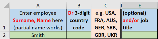
- not only look into $B$2, but $B$2:$B$6 (for each of the cells independently; some may be blank but others will have an entry)
- not only look into $E$2, but $E$2:$E$6 (for each of the cells independently; some may be blank but others will have an entry)
- not only look into $A$2, but $A$2:$A$6 (for each of the cells independently; some may be blank but others will have an entry)

 

[etaf]

i don't follow completely
You are checking an Array with an IF ( Isblank()

then doing 2 different sums if TRUE or FALSE

=IF(ISBLANK($A$2:$A$6),
TRUE
SUMIFS('Labor report'!$N$2:$N$200000, 'Labor report'!$AB$2:$AB$200000,"*" & $B$2 & "*",'Labor report'!$L$2:$L$200000,"*" & $E$2 & "*",'Labor report'!$B$2:$B$200000,E$15,'Labor report'!$D$2:$D$200000,$B16),
FALSE
SUMIFS('Labor report'!$N$2:$N$200000, 'Labor report'!$K$2:$K$200000,"*" & $A$2 & "*",'Labor report'!$B$2:$B$200000,E$15,'Labor report'!$D$2:$D$200000,$B16))

So IF A2 is Blank, then use the first formula
But I suspect you also want to test to see if
B2 & E2 is blank

IS this and AND needed

=AND( ISBLANK(A2),ISBLANK(B2),ISBLANK(E2) ) type of formula
OR a counta() count cells that are not empty

Sorry i'm not following the requirement
Can you give a little more detail
maybe a matrix
Depending on what cells A,B,E are blank

 

[virtuosok]

Thanks etaf,
In terms of checks for blanks, I only need to check for A2:A6; for subsequent calc it doesn't matter much if other cells are blank or not. The formula as it stands now works for my needs - I just need to expand the selection for B2, E2, and A2 into B2:B6, E2:E6, and A2:A6, accordingly. To put it differently, I used to have only row 2 for inputs, now I added rows 3-6 to cover more scenarios at the same time... need to tweak the above formula accordingly.

Hope this makes sense.
OR, let me make it less complicated. For this piece
SUMIFS('Labor report'!$N$2:$N$200000, 'Labor report'!$K$2:$K$200000,"*" & $A$2 & "*",'Labor report'!$B$2:$B$200000,E$15,'Labor report'!$D$2:$D$200000,$B16)
How can I calculate total SUMIFS not only for A2 (as it currently stands), but also for A3, A4, A5, and A6 so that they all are verified independently and then added up?

 

[jasonb75]

That is nothing like the requirement vaguely implied by your original post.

See if this works, it is what you have now asked for, but I have my doubts that it is what you need.

=SUM(SUMIFS('Labor report'!$N$2:$N$200000, 'Labor report'!$AB$2:$AB$200000,"*" & $B$2:$B$6 & "*",'Labor report'!$L$2:$L$200000,"*" & $E$2:$E$6 & "*",'Labor report'!$K$2:$K$200000,"*" & $A$2:$A$6 & "*"'Labor report'!$B$2:$B$200000,E$15,'Labor report'!$D$2:$D$200000,$B16))

 

[virtuosok]

Apologies for my complicated explanation, give me another chance...
This is what I had initially and it worked perfectly for my purposes:

The formula was as follows:
=IF(ISBLANK($A$2),SUMIFS('Labor report'!$N$2:$N$200000, 'Labor report'!$AB$2:$AB$200000,"*" & $B$2 & "*",'Labor report'!$L$2:$L$200000,"*" & $E$2 & "*",'Labor report'!$B$2:$B$200000,E$14,'Labor report'!$D$2:$D$200000,$B15),SUMIFS('Labor report'!$N$2:$N$200000, 'Labor report'!$K$2:$K$200000,"*" & $A$2 & "*",'Labor report'!$B$2:$B$200000,E$14,'Labor report'!$D$2:$D$200000,$B15))
In other words, if there was a name/surname in cell A2, the formula would do the calc with it; otherwise it would do the calc based on entries in cells B2 and E2 (if anything there).
Now I would need to do analysis based on several inputs and not just one; these will be either in cells A2:A6, or in cells B2:B6 and E2:E6. There might be all 5 cells in the range with a condition, or only some of them.
Scenario 1:

Do I do SUM(SUMIFS A2, SUMIFS A3, SUMIFS A4, SUMIFS A5, SUMIFS A6), or SUM(SUMIFS A2:A6), or SUMIFS A2 + SUMIFS A3... or is there another rule I need to try? Same for
Scenario 2:

 

[jasonb75]

Trying to simplify this a bit, are you looking for all possible combinations? For example, if the criteria were entered as in rows 2 and 3 below, should the formula be looking at all of the combinations listed from row 6?

22.04.21.xlsx
	A	B	C
1	Name	Code	Title
2	Smith	AUS	Manager
3	Jones	USA	Cleaner
4
5	All combinations
6	Smith	AUS	Manager
7	Smith	USA	Manager
8	Jones	AUS	Manager
9	Jones	USA	Manager
10	Smith	AUS	Cleaner
11	Smith	USA	Cleaner
12	Jones	AUS	Cleaner
13	Jones	USA	Cleaner
Sheet3

 

[virtuosok]

No, there are actually less combinations that I'm after.
In the above example, columns A, B, and C won't have entries at the same time. It will be either A, or alternatively, B&C. But, some of the cells in a given column might be blank, so I don't want this condition to be counted twice. In other words, the two "scenarios" with screenshots that I posted above are mutually exclusive.
I'm also posting blinded workbook that I'm working with
Blinded report v4.0.xlsm
The formulas which I'm trying to develop belong to cells E15:M67 on tab Calc

 

[jasonb75]

I haven't tested this formula, there are still a couple of grey areas in the requirement.

As you're using excel 2016, this must be array confirmed with Ctrl Shift Enter.

=SUM(IF(ISBLANK($A$2:$A$6),SUMIFS('Labor report'!$N$2:$N$200000, 'Labor report'!$AB$2:$AB$200000,"*" & $B$2:$B$6 & "*",'Labor report'!$L$2:$L$200000,"*" & $E$2:$E$6 & "*",'Labor report'!$B$2:$B$200000,E$15,'Labor report'!$D$2:$D$200000,$B16),SUMIFS('Labor report'!$N$2:$N$200000, 'Labor report'!$K$2:$K$200000,"*" & $A$2:$A$6 & "*",'Labor report'!$B$2:$B$200000,E$15,'Labor report'!$D$2:$D$200000,$B16)))

edit:- a second option, that would work slightly differently to the first. Still needs to be array confirmed.

=SUM(IF(ISBLANK($A$2:$A$6),SUMIFS('Labor report'!$N$2:$N$200000, 'Labor report'!$AB$2:$AB$200000,"*" & $B$2:$B$6 & "*",'Labor report'!$L$2:$L$200000,"*" & TRANSPOSE($E$2:$E$6) & "*",'Labor report'!$B$2:$B$200000,E$15,'Labor report'!$D$2:$D$200000,$B16),SUMIFS('Labor report'!$N$2:$N$200000, 'Labor report'!$K$2:$K$200000,"*" & $A$2:$A$6 & "*",'Labor report'!$B$2:$B$200000,E$15,'Labor report'!$D$2:$D$200000,$B16)))

 

[virtuosok]

Thank you jasonb75! This is very close to what I need. Two comments only:
1. For range $A$2:$A$6, the formula works impeccably for my needs only when all cells, from A2 to A6, have some inputs. Otherwise if one (or more) of these cells are empty, outputs are incorrect as I am getting a much higher total than expected.
2. For ranges in columns B and E, it's the same problem, but since these are 2 columns it's a bit more complicated to explain. Let's see if we can fix A column and then I may be able to replicate the solution for B and E...

 

[jasonb75]

Are the wildcards needed on all 3 ranges?
I suspect that they are the biggest part of the problem.