help with If and formula

[Samgraphics]

HI,
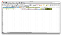
So I’m trying to find a more efficient way to achieve this results. I used an if an function to see if the value in a cell is an odd or an even number and is less than ten. If it is it will highlight that cell with the color I choose. I made the column letter absolute so that I can copy the formula down the column. But I also want it to check that same column to see if the value is odd and greater than 10, is even and less than ten and is even and greater than ten and apply a specific background color for which ever is true. So that requires four different formulas. Not only that but I want it to do that for an array of 5 numbers, one in each column. So in total I have to write that formula 20 times for one row. I’m using excel’s conditional formatting to achieve this with the use formula to determine results option. The good thing is I can then copy it down to all the other arrays of numbers. I’m just worried that it will make excel run too slow since I have over 300,000 arrays of numbers.

In addition each cell has another formula that checks to see if the value is odd or even and less than or greater than 10 and adds a text string of odd or even in each each column using the if and formula.

Also in a separate two columns I’m using sumproduct(mod()) to check how many odds and evens there are in the row.

I tried to upload a minisheet but it didn't work on my mac.

Is there a more efficient way to accomplish this?

Thanks in advance

 

[StephenCrump]

It's not clear what the end-game here is ...

You can conditionally format the entire range using only three formulae (plus a default background colour that will show only if the 4th option applies - I've used yellow below).

But is conditional formatting going to be of any practical use? The range is way too big to visualise, and you can't (readily) filter or search by cell colour.

Would it make more sense to convert to numeric values 1-4 so you can easily count, filter etc?

	A	B	C	D	E	F	G	H	I	J	K
1	N	10
2
3	1	Odd/Small
4	2	Even/Small
5	3	Odd/Large
6	4	Even/Large
7
8	Sample						Result
9	13	10	3	13	5		3	2	1	3	1
10	13	14	15	2	10		3	4	3	2	2
11	5	8	7	10	18		1	2	1	2	4
12	15	10	12	15	9		3	2	4	3	1
13	9	15	7	16	13		1	3	1	4	3
14	14	4	13	7	17		4	2	3	1	3
15	9	12	5	15	11		1	4	1	3	3
16	1	18	8	7	10		1	4	2	1	2
17	16	6	8	18	7		4	2	2	4	1
Sheet1

Cell Formulas
Range	Formula
G9:K17	G9	=IF(ISODD(A9),1,2)+2*(A9>N)

Named Ranges
Name	Refers To	Cells
N	=Sheet1!$B$1	G9:K17

Cells with Conditional Formatting
Cell	Condition		Cell Format	Stop If True
A9:E17	Expression	=AND(ISODD(A9),A9<N)	text	NO
A9:E17	Expression	=A9<N	text	NO
A9:E17	Expression	=ISODD(A9)	text	NO

 

[Samgraphics]

It's not clear what the end-game here is ...

You can conditionally format the entire range using only three formulae (plus a default background colour that will show only if the 4th option applies - I've used yellow below).

But is conditional formatting going to be of any practical use - the range is way too big to visualise, and you can't (readily) filter or search by cell colour.

Would it make more sense to convert to numeric values 1-4 so you can easily count, filter etc?

	A	B	C	D	E	F	G	H	I	J	K
1	N	10
2
3	1	Odd/Small
4	2	Even/Small
5	3	Odd/Large
6	4	Even/Large
7
8	Sample						Result
9	13	10	3	13	5		3	2	1	3	1
10	13	14	15	2	10		3	4	3	2	2
11	5	8	7	10	18		1	2	1	2	4
12	15	10	12	15	9		3	2	4	3	1
13	9	15	7	16	13		1	3	1	4	3
14	14	4	13	7	17		4	2	3	1	3
15	9	12	5	15	11		1	4	1	3	3
16	1	18	8	7	10		1	4	2	1	2
17	16	6	8	18	7		4	2	2	4	1
Sheet1

Cell Formulas
Range	Formula
G9:K17	G9	=IF(ISODD(A9),1,2)+2*(A9>N)

Named Ranges
Name	Refers To	Cells
N	=Sheet1!$B$1	G9:K17

Cells with Conditional Formatting
Cell	Condition		Cell Format	Stop If True
A9:E17	Expression	=AND(ISODD(A9),A9<N)	text	NO
A9:E17	Expression	=A9<N	text	NO
A9:E17	Expression	=ISODD(A9)	text	NO

Hi Stephen, thank you so much for the quick response and for the time in helping me out.

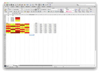
what you described here makes perfect sense. I understand the idea. The problem is I don't really understand the code and I get the conditional formatting part of it. The part I don't get is how to convert to numeric values. When I copied the code from the xl2bb I'm getting a #NAME error and I don't know how to fix it. I attached a screenshot. But what you said is what I'm looking for it's just that my excel skill level is subpar at best.
So what I'm trying to do is find out the number of odds/even in each row, and also return in separate columns whether the number in each cell is a low/high odd/even and color code them to represent it visually. I would like it to return a value just like you did in the example where it returned numbers that represent high/low odd/even but I'd like the conditional formatting to be in the returned cells and I'd like to change it from numbers to text. Numbers get jumbled up in my brain very easily that's why I was looking for a more visual representation of the data, it will also help with spotting patterns.

The end game here is that it's easier for me to visualize with colors and text since the numbers repeat so often sometimes my brain skips row and I end up mixing up the numbers. The numeric values for being able to filter search etc makes much more logical sense but like I said my excel skills are very poor.

I'm probably not making much sense here, sorry.

 

[Alex Blakenburg]

When I copied the code from the xl2bb I'm getting a #NAME error and I don't know how to fix it.

XL2BB is not transferring the Named Range and @StephenCrump has one in his spreadsheet. This is what is causing the #NAME error.
Easiest way to fix it is

• click on B2 (it has a value of 10 in the Cell).
• Then in the address box in the top left corner where it says B2, type in N and hit return.
  All the #NAME references should disappear

(I wouldn't normally use such a cryptic range name but that is what is being used by the XL2BB worksheet)

 

[StephenCrump]

So perhaps more like this:

	A	B	C	D	E	F	G	H	I	J	K	L	M	N	O
1	Boundary	10
2
3	Sample						Odds	Evens		Result
4	13	10	3	13	5		4	1		ODD/LARGE	EVEN/SMALL	ODD/SMALL	ODD/LARGE	ODD/SMALL
5	13	14	15	2	10		2	3		ODD/LARGE	EVEN/LARGE	ODD/LARGE	EVEN/SMALL	EVEN/SMALL
6	5	8	7	10	18		2	3		ODD/LARGE	EVEN/SMALL	ODD/SMALL	EVEN/SMALL	EVEN/LARGE
7	15	10	12	15	9		3	2		ODD/LARGE	EVEN/SMALL	EVEN/LARGE	ODD/LARGE	ODD/SMALL
8	9	15	7	16	13		4	1		ODD/LARGE	ODD/LARGE	ODD/SMALL	EVEN/LARGE	ODD/LARGE
9	14	4	13	7	17		3	2		EVEN/LARGE	EVEN/SMALL	ODD/LARGE	ODD/SMALL	ODD/LARGE
10	9	12	5	15	11		4	1		ODD/LARGE	EVEN/LARGE	ODD/SMALL	ODD/LARGE	ODD/LARGE
11	1	18	8	7	10		2	3		ODD/LARGE	EVEN/LARGE	EVEN/SMALL	ODD/SMALL	EVEN/SMALL
12	16	6	8	18	7		1	4		EVEN/LARGE	EVEN/SMALL	EVEN/SMALL	EVEN/LARGE	ODD/SMALL
13
Sheet1

Cell Formulas
Range	Formula
G4:G12	G4	=SUMPRODUCT(MOD(A4:E4,2))
H4:H12	H4	=COLUMNS(A4:E4)-G4
J4:N12	J4	=IF(ISODD(A4),"ODD","EVEN")&"/" & IF(A4>$B$1,"LARGE","SMALL")

Cells with Conditional Formatting
Cell	Condition		Cell Format	Stop If True
J4:N12	Cell Value	="EVEN/LARGE"	text	NO
J4:N12	Cell Value	="ODD/LARGE"	text	NO
J4:N12	Cell Value	="EVEN/SMALL"	text	NO
J4:N12	Cell Value	="ODD/SMALL"	text	NO

Thanks Alex for explaining the named range. I've used a cell reference $B$1 here instead.

 

[Samgraphics]

So perhaps more like this:

	A	B	C	D	E	F	G	H	I	J	K	L	M	N	O
1	Boundary	10
2
3	Sample						Odds	Evens		Result
4	13	10	3	13	5		4	1		ODD/LARGE	EVEN/SMALL	ODD/SMALL	ODD/LARGE	ODD/SMALL
5	13	14	15	2	10		2	3		ODD/LARGE	EVEN/LARGE	ODD/LARGE	EVEN/SMALL	EVEN/SMALL
6	5	8	7	10	18		2	3		ODD/LARGE	EVEN/SMALL	ODD/SMALL	EVEN/SMALL	EVEN/LARGE
7	15	10	12	15	9		3	2		ODD/LARGE	EVEN/SMALL	EVEN/LARGE	ODD/LARGE	ODD/SMALL
8	9	15	7	16	13		4	1		ODD/LARGE	ODD/LARGE	ODD/SMALL	EVEN/LARGE	ODD/LARGE
9	14	4	13	7	17		3	2		EVEN/LARGE	EVEN/SMALL	ODD/LARGE	ODD/SMALL	ODD/LARGE
10	9	12	5	15	11		4	1		ODD/LARGE	EVEN/LARGE	ODD/SMALL	ODD/LARGE	ODD/LARGE
11	1	18	8	7	10		2	3		ODD/LARGE	EVEN/LARGE	EVEN/SMALL	ODD/SMALL	EVEN/SMALL
12	16	6	8	18	7		1	4		EVEN/LARGE	EVEN/SMALL	EVEN/SMALL	EVEN/LARGE	ODD/SMALL
13
Sheet1

Cell Formulas
Range	Formula
G4:G12	G4	=SUMPRODUCT(MOD(A4:E4,2))
H4:H12	H4	=COLUMNS(A4:E4)-G4
J4:N12	J4	=IF(ISODD(A4),"ODD","EVEN")&"/" & IF(A4>$B$1,"LARGE","SMALL")

Cells with Conditional Formatting
Cell	Condition		Cell Format	Stop If True
J4:N12	Cell Value	="EVEN/LARGE"	text	NO
J4:N12	Cell Value	="ODD/LARGE"	text	NO
J4:N12	Cell Value	="EVEN/SMALL"	text	NO
J4:N12	Cell Value	="ODD/SMALL"	text	NO

Thanks Alex for explaining the named range. I've used a cell reference $B$1 here instead.

Hi Stephen,
YES YES YES, that's exactly what I was looking for thank you so much. Huge help on this.
thanks so much.
Also, a big thank you to Alex also, your suggestion did solve the issue I was having with the error as well. Thank you.

There is just a small issue. For the conditional formatting, was I supposed to type in the formula (="EVEN/LARGE") "use formula to determine which cells to format" or select or "format only cells that contain" and select "specific text"? When I enter the formula above under "use formula to determine ...." nothing happens. No error but the formatting doesn't work. It only works when I select "specific text", which is ok. I was just wondering if I was doing something wrong.

However, the other codes work like a charm.
thanks again.

If I'm not being too much of a pain I'd like to ask for help with one other issue that just came up while I was using the very efficient code you gave me.

I was wondering if you could help.
I am trying to rate the numbers. Say for example a number has 1 low odd, 2 high odds, and 2 high evens I would like to put a ratting in the column next to it like "good" if I think that's a good combination or "bad" if I think it's a bad combination. So I'm trying to see if there is a way to check/filter the results to see how man odds/even and low/high in each 5 numbers or is that too much? Something like =IF(C2:E2="LOW ODD"*2&"HIGH ODD"*1&"HIGH EVEN"*2,"GOOD","BAD") I know I can't use SUMPRODUCT because the value in each cell is not a number but I'm lost as to how to solve this.

Thank you again for all your help.

 

[StephenCrump]

There is just a small issue. For the conditional formatting, was I supposed to type in the formula (="EVEN/LARGE") "use formula to determine which cells to format" or select or "format only cells that contain" and select "specific text"? When I enter the formula above under "use formula to determine ...." nothing happens. No error but the formatting doesn't work. It only works when I select "specific text", which is ok. I was just wondering if I was doing something wrong.

I did it this way:

Or you could use a formula: =J4="EVEN/LARGE"

I am trying to rate the numbers. Say for example a number has 1 low odd, 2 high odds, and 2 high evens I would like to put a ratting in the column next to it like "good" if I think that's a good combination or "bad" if I think it's a bad combination. So I'm trying to see if there is a way to check/filter the results to see how man odds/even and low/high in each 5 numbers or is that too much? Something like =IF(C2:E2="LOW ODD"*2&"HIGH ODD"*1&"HIGH EVEN"*2,"GOOD","BAD") I know I can't use SUMPRODUCT because the value in each cell is not a number but I'm lost as to how to solve this.

You can use the COUNTIF and/or COUNTIFS functions to count how many EVEN/LARGE's etc that you have.

If you let us know which combinations are GOOD and which are BAD, it should be easy to write an appropriate formula.

 

[Samgraphics]

I did it this way:

View attachment 55651

Or you could use a formula: =J4="EVEN/LARGE"


You can use the COUNTIF and/or COUNTIFS functions to count how many EVEN/LARGE's etc that you have.

If you let us know which combinations are GOOD and which are BAD, it should be easy to write an appropriate formula.

HI STEPHEN SO SORRY FOR THE LATE REPLY. I NEVER NOTICED THE NOTIFICATION IN MY INBOX. ANYWAY, I WAS ABLE TO FIGURE THAT PART OUT AFTER PLAYING AROUND FOR A BIT. THANK YOU SO MUCH. YOU'VE BEEN SUCH A BIG HELP.
I HAVE BEEN PLAYING AROUND WITH THE FORMULA YOU WROTE TO HELP ME UNDERSTAND IT BETTER AND I WAS WONDERING IF IT'S NOT TOO MUCH TROUBLE IF YOU COULD PLEASE HELP ME OUT SOME MORE.

I'VE ADJUSTED THE FORMULA A BIT TO THIS
=IF(C2>$AF$3,"HIGH","LOW")&" "&IF(C2>$AF$2,"HIGH","LOW")&" " & IF(ISODD(C2),"ODD","EVEN")
AS YOU CAN SEE I ADDED ANOTHER WORD AND CHANGED THE "/? TO A SPACE. WHAT I'M TRYING TO DO IS THIS, SEE SCREENGRAB.
NUMBERS THAT ARE LOWER THAN 10 ARE "LOW LOW + ODD/EVEN"
GREATER THAN 10 BUT LESS THAN 18 ARE "HIGH LOW + ODD/EVEN"
GREATER THAN 18 BUT LESS THAN 27 ARE "LOW HIGH + ODD/EVEN"
AND GREATER THAN 27 ARE "HIGH HIGH + ODD/EVEN"

I'VE ALREADY FIGURED OUT THE "LOW LOW" AND THE "HIGH LOW" BUT I CAN'T FIGURE OUT THE "HIGH HIGH" AND THE "LOW HIGH" I'M GUESSING IT NEEDS TO BE AN IF/OR STATEMENT?

PLEASE HELP ME.
THANK YOU SO MUCH

 

[StephenCrump]

You could use VLOOKUP for this:

	A	B	C	D	E	F	G	H	I	J	K
1	Table
2	0	LOW LOW
3	10	HIGH LOW
4	18	LOW HIGH
5	27	HIGH HIGH
6	Sample						Results
7	24	5	5	26	25		LOW HIGH EVEN	LOW LOW ODD	LOW LOW ODD	LOW HIGH EVEN	LOW HIGH ODD
8	4	25	12	26	2		LOW LOW EVEN	LOW HIGH ODD	HIGH LOW EVEN	LOW HIGH EVEN	LOW LOW EVEN
9	15	24	20	7	3		HIGH LOW ODD	LOW HIGH EVEN	LOW HIGH EVEN	LOW LOW ODD	LOW LOW ODD
10	16	9	13	17	4		HIGH LOW EVEN	LOW LOW ODD	HIGH LOW ODD	HIGH LOW ODD	LOW LOW EVEN
11	31	17	11	29	19		HIGH HIGH ODD	HIGH LOW ODD	HIGH LOW ODD	HIGH HIGH ODD	LOW HIGH ODD
12	22	20	17	18	9		LOW HIGH EVEN	LOW HIGH EVEN	HIGH LOW ODD	LOW HIGH EVEN	LOW LOW ODD
13	19	9	17	14	29		LOW HIGH ODD	LOW LOW ODD	HIGH LOW ODD	HIGH LOW EVEN	HIGH HIGH ODD
14	29	22	24	14	25		HIGH HIGH ODD	LOW HIGH EVEN	LOW HIGH EVEN	HIGH LOW EVEN	LOW HIGH ODD
15	19	14	24	23	22		LOW HIGH ODD	HIGH LOW EVEN	LOW HIGH EVEN	LOW HIGH ODD	LOW HIGH EVEN
Sheet1

Cell Formulas
Range	Formula
G7:K15	G7	=VLOOKUP(A7,$A$2:$B$5,2,1)&IF(ISODD(A7)," ODD"," EVEN")

It's not clear where the boundaries are? If 10 is LOW LOW, just change cell A3 from 10 to 11.

PS: Sorry this reply is late ... I've been away a couple of weeks.

 

[Samgraphics]

Hi Stephen, that's ok, and thank you for replying anyway. I really appreciate it because, while someone else gave me a formula,
=IF(C2>$AF$4,"HIGH HIGH",IF(C2>$AF$3,"LOW HIGH",IF(C2>$AF$2,"HIGH LOW","LOW LOW")))&" " &IF(ISODD(C2),"ODD","EVEN")
this vlookup is so much more robust and shorter.
Thank you so much