Help with Index/Match for multiple criteria within a date range

[hope2022]

Hi! I'm pretty comfortable with ifs and vlookup, but these formulas are not providing the results I am looking for. I am thinking I should use Index/Match, but I am less familiar with these and arrays.

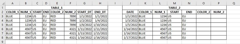
I want to match COLOR_1, NUM_1, START, END from TABLE_2 on TABLE_1, and return values for COLOR_2 and NUM_2 from TABLE_1 onto TABLE_2. This could be an easy concatenate and vlookup, but then I also only want to return results with matches but also where the DATE from TABLE_2 matches or falls within the START_DT and END_DT from TABLE_1.

Any help or guidance would be appreciated!

 

[KRice]

Here is one approach for Excel 365 using named tables (Ctrl-t when in the data, confirm the correct range including headers, and then change name to TABLE_1 or TABLE_2) and structured references. If more than one match is returned on a row, this will generate a #SPILL! error. Do you anticipate multiple matches for any row?

MrExcel_20220315.xlsx
	A	B	C	D	E	F	G	H	I	J	K	L	M	N	O	P
1	TABLE_1									TABLE_2
2	COLOR_1	NUM_1	START	END	COLOR_2	NUM_2	START_DT	END_DT		DATE	COLOR_1	NUM_1	START	END	COLOR_2	NUM_2
3	BLUE	1234	US	EU	RED	7890	1/1/2022	1/1/2022		1/1/2022	BLUE	1234	US	EU	RED	7890
4	BLUE	1234	US	EU	RED	7890	1/2/2022	1/4/2022		1/3/2022	BLUE	1234	US	EU	RED	7890
5	BLUE	1234	US	EU	RED	7890	1/6/2022	1/10/2022		1/5/2022	BLUE	1234	US	EU
6	BLUE	4567	US	EU	RED	4321	1/11/2022	1/11/2022		1/14/2022	BLUE	4567	US	EU	RED	4321
7	BLUE	4567	US	EU	RED	4321	1/13/2022	1/15/2022		1/16/2022	BLUE	4567	US	EU	RED	4321
8	BLUE	4567	US	EU	RED	4321	1/16/2022	1/16/2022		1/17/2022	BLUE	4567	US	EU
Sheet11

Cell Formulas
Range	Formula
O3:O8	O3	=FILTER(TABLE_1[COLOR_2],(TABLE_1[COLOR_1]=[@[COLOR_1]])*(TABLE_1[NUM_1]=[@[NUM_1]])*(TABLE_1[START]=[@START])*(TABLE_1[END]=[@END])*(TABLE_1[START_DT]<=[@DATE])*(TABLE_1[END_DT]>=[@DATE]),"")
P3:P8	P3	=FILTER(TABLE_1[NUM_2],(TABLE_1[COLOR_1]=[@[COLOR_1]])*(TABLE_1[NUM_1]=[@[NUM_1]])*(TABLE_1[START]=[@START])*(TABLE_1[END]=[@END])*(TABLE_1[START_DT]<=[@DATE])*(TABLE_1[END_DT]>=[@DATE]),"")

 

[hope2022]

Here is one approach for Excel 365 using named tables (Ctrl-t when in the data, confirm the correct range including headers, and then change name to TABLE_1 or TABLE_2) and structured references. If more than one match is returned on a row, this will generate a #SPILL! error. Do you anticipate multiple matches for any row?

MrExcel_20220315.xlsx
	A	B	C	D	E	F	G	H	I	J	K	L	M	N	O	P
1	TABLE_1									TABLE_2
2	COLOR_1	NUM_1	START	END	COLOR_2	NUM_2	START_DT	END_DT		DATE	COLOR_1	NUM_1	START	END	COLOR_2	NUM_2
3	BLUE	1234	US	EU	RED	7890	1/1/2022	1/1/2022		1/1/2022	BLUE	1234	US	EU	RED	7890
4	BLUE	1234	US	EU	RED	7890	1/2/2022	1/4/2022		1/3/2022	BLUE	1234	US	EU	RED	7890
5	BLUE	1234	US	EU	RED	7890	1/6/2022	1/10/2022		1/5/2022	BLUE	1234	US	EU
6	BLUE	4567	US	EU	RED	4321	1/11/2022	1/11/2022		1/14/2022	BLUE	4567	US	EU	RED	4321
7	BLUE	4567	US	EU	RED	4321	1/13/2022	1/15/2022		1/16/2022	BLUE	4567	US	EU	RED	4321
8	BLUE	4567	US	EU	RED	4321	1/16/2022	1/16/2022		1/17/2022	BLUE	4567	US	EU
Sheet11

Cell Formulas
Range	Formula
O3:O8	O3	=FILTER(TABLE_1[COLOR_2],(TABLE_1[COLOR_1]=[@[COLOR_1]])*(TABLE_1[NUM_1]=[@[NUM_1]])*(TABLE_1[START]=[@START])*(TABLE_1[END]=[@END])*(TABLE_1[START_DT]<=[@DATE])*(TABLE_1[END_DT]>=[@DATE]),"")
P3:P8	P3	=FILTER(TABLE_1[NUM_2],(TABLE_1[COLOR_1]=[@[COLOR_1]])*(TABLE_1[NUM_1]=[@[NUM_1]])*(TABLE_1[START]=[@START])*(TABLE_1[END]=[@END])*(TABLE_1[START_DT]<=[@DATE])*(TABLE_1[END_DT]>=[@DATE]),"")

Hi! Thanks for the great reply!

Your formulas were not working for me, but I achieved similar results with

R3 =INDEX(E$3:E$8,SUMPRODUCT((M3>=G$3:G$8)*(M3<=H$3:H$8)*MATCH(1,(N3=A$3:A$8)*(O3=B$3:B$8)*(P3=C$3:C$8)*(Q3=D$3:D$8),0)))
S3 =INDEX(F$3:F$8,SUMPRODUCT((M3>=G$3:G$8)*(M3<=H$3:H$8)*MATCH(1,(N3=A$3:A$8)*(O3=B$3:B$8)*(P3=C$3:C$8)*(Q3=D$3:D$8),0)))
Ideally there should not be duplicates, because the date ranges should not overlap. So while there may be several rows with the same COLOR_1, NUM_1, START and END, they should still be unique rows due to the START_DT and END_DT

There may be cases where there are gaps in the dates though, so some records should not find a COLOR_2 or NUM_2 if there the DATE does not fall within the START_DT and END_DT

I hope that I am making sense!

Thanks!

 

[KRice]

Your formulas were not working for me

From your latest post, it appears you are using conventional references to cell ranges. My offering assumed the data existed in a formal table, where an entire column can be referenced using the column header name (that's what my earlier comment about "Ctrl-t..." referred to). Do your data exist in a formal table? Are you using Excel 365? I'm trying to understand what type of issue you encountered.

 

[KRice]

The SUMPRODUCT formula in your post #3 does not correspond to the table presented. For example, the date in Table2 is not described in the formulas. Additionally, the use of SUMPRODUCT like this will not return the correct match. You are multiplying two arrays together and then summing the results. If you happen to have {0;0;1;0;0;0} and {1;1;1;1;1;1}, then only the 3rd row of Table 1 satisfies the date criteria and all rows of Table2 satisfy the other non-date criteria (indicated by 1's in the arrays), then when SUMPRODUCT operates on these two arrays, it will yield an answer of 1...but we can see that only the 3rd row satisfies all criteria. So SUMPRODUCT is returning the number of rows where all criteria are met, but that is not the same as the relative position of the matching rows in the table. Consequently, your result will be taken from the first row of Table1, which is not correct.

You don't need SUMPRODUCT in this case. Instead, bring the date criteria inside the MATCH function. Be aware that using MATCH will return only the first instance where the criteria are met. Here is a revised version with cell ranges that match the tables presented, and with all criteria pulled inside the MATCH function. Note the first row of the table is an example to illustrate the point in the previous paragraph. In this example, the two arrays are {0;0;1;0;0;0} and {1;1;1;0;0;0} (so only the 3rd row matches the date criteria and rows 1,2,and 3 match the other non-date criteria). The correct answer is Purple from the 3rd row, but there is only one matching row, so SUMPRODUCT returns 1 and you get the color from the first row of Table1...which is not correct. The formula presented on row 4 should return the first match from Table1 where all criteria are satisfied.

MrExcel20220321.xlsx
	A	B	C	D	E	F	G	H	I	J	K	L	M	N	O	P
1	TABLE_1									TABLE_2
2	COLOR_1	NUM_1	START	END	COLOR_2	NUM_2	START_DT	END_DT		DATE	COLOR_1	NUM_1	START	END	COLOR_2	NUM_2
3	BLUE	1234	US	EU	RED	7890	1/1/2022	1/1/2022		1/8/2022	BLUE	1234	US	EU	RED	<--Wrong answer
4	BLUE	1234	US	EU	GREEN	7890	1/1/2022	1/4/2022		1/3/2022	BLUE	1234	US	EU	GREEN	7890
5	BLUE	1234	US	EU	PURPLE	7890	1/6/2022	1/10/2022		1/5/2022	BLUE	1234	US	EU
6	BLUE	4567	US	EU	YELLOW	4321	1/11/2022	1/11/2022		1/14/2022	BLUE	4567	US	EU	ORANGE	4321
7	BLUE	4567	US	EU	ORANGE	4321	1/13/2022	1/15/2022		1/16/2022	BLUE	4567	US	EU	BROWN	4321
8	BLUE	4567	US	EU	BROWN	4321	1/16/2022	1/16/2022		1/17/2022	BLUE	4567	US	EU
Sheet3

Cell Formulas
Range	Formula
O3	O3	=INDEX(E$3:E$8,SUMPRODUCT((J3>=G$3:G$8)*(J3<=H$3:H$8)*MATCH(1,(K3=A$3:A$8)*(L3=B$3:B$8)*(M3=C$3:C$8)*(N3=D$3:D$8),0)))
O4:O8	O4	=IFERROR(INDEX($E3:$E8,MATCH(1,($J4>=$G3:$G8)*($J4<=$H3:$H8)*($K4=$A3:$A8)*($L4=$B3:$B8)*($M4=$C3:$C8)*($N4=$D3:$D8),0)),"")
P4:P8	P4	=IFERROR(INDEX($F3:$F8,MATCH(1,($J4>=$G3:$G8)*($J4<=$H3:$H8)*($K4=$A3:$A8)*($L4=$B3:$B8)*($M4=$C3:$C8)*($N4=$D3:$D8),0)),"")

 

[KRice]

Sorry, I didn't get my previous response edited in time...
The MATCH inside the SUMPRODUCT formula is not returning an array (as I incorrectly stated in my last post). It is returning the location of the first match for the non-date criteria. When that number is multiplied by the matching-date array with SUMPPRODUCT, you will obtain an answer that is not necessarily correct. The main point is to incorporate the criteria inside MATCH and not use SUMPRODUCT.