Help with Index + Vlookup + multiple criteria including checkboxes across 2 tabs

[GameofFormulas]

Need help with a complex formula. I've been trying to figure it to no avail.

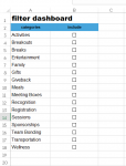
Tab 1 (filter dashboard) shows 16 different categories that appear in column A on tab 3 (complete data). Each category has a corresponding checkbox. I have already cell linked each checkbox so TRUE / FALSE appears for criteria purposes - I've just changed the text color to white so you don't see TRUE/FALSE. I would like for the data on tab 3 to be filtered and appear on tab 2 (filtered results) based on which checkboxes are checked on tab 1.

Note:

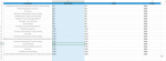
• Each line-item on Tab 3 (complete data) can have 1 or more categories or "tags". The applicable categories for each line-item are shown in Column A and are comma separated.
• Tab 3 (complete data) just shows dummy data except for the category column (A).

Appreciate your help!

 

[braindiesel]

Here is my solution...

Book4
	A	B	C	D	E	F	G	H	I	J	K
1		TAB ONE	ADD THIS FORMULA		Create this named range			TAB 3 Column A	Col E Referencing Column A	Column F Tab 3	Column G Tab 3
2	Cat	TRUE	1		Cat			Dog	FALSE	0	2
3	Dog	FALSE	0		Bunny			Giraffe, Bunny	TRUE	2	4
4	Bunny	TRUE	3		Fish			Dog, Bird, Hamster	FALSE	0
5	Bird	FALSE	0		Label 7			Cat Fish	TRUE	4
6	Fish	TRUE	5		Label 9
7	Hamster	FALSE	0		Label 11
8	Label 7	TRUE	7		Label 13			On Tab 2 in cell A2
9	Label 8	FALSE	0					Giraffe, Bunny
10	Label 9	TRUE	9					Cat Fish
11	Label 10	FALSE	0						For the remaining columns you can adjust this formula to be looking at Tab 3 column B, C, & D
12	Label 11	TRUE	11
13	Label 12	FALSE	0
14	Label 13	TRUE	13
15	Label 14	FALSE	0
Sheet1

Cell Formulas
Range	Formula
I2:I5	I2	=SUMPRODUCT(--ISNUMBER(SEARCH(myCats,H2)))>0
J2:J5,C2:C15	J2	=(I2=TRUE)*ROW(H1)
K2:K3	K2	=IF(COUNTIF($J$2:$J$5,">"&0)>=ROWS($J$2:J2),SMALL($J$2:$J$5,ROWS($J$2:J2)+COUNTIF($J$2:$J$5,0)),"")
K4:K5	K4	=IF(COUNTIF($J$2:$J$5,">"&0)>=ROWS($J$2:J4),INDEX($H$2:$H$5,SMALL($J$2:$J$5,ROWS($J$2:J4)+COUNTIF($J$2:$J$5,0)),1),"")
H9:H12	H9	=IF(ROW(A1)<=COUNT(K:K),INDEX($H$2:$H$5,SMALL(K:K,ROW(A1)),1),"")
E2:E15	E2	=IF(COUNTIF($C$2:$C$15,">"&0)>=ROWS($E$2:E2),INDEX($A$2:$A$15,SMALL($C$2:$C$15,ROWS($E$2:E2)+COUNTIF($C$2:$C$15,0)),1),"")

Named Ranges
Name	Refers To	Cells
myCats	=OFFSET(Sheet1!$E$1,1,0,COUNTIF(Sheet1!$C$2:$C$15,">"&0),1)	E2:E15

I2 formula courtesy of this google search result...
Excel formula: Cell contains one of many things | Exceljet

 

[GameofFormulas]

Thanks, BrainDiesel! I really appreciate your help.

Working through your instructions and got stuck on the difference in formulas for K2:K3 & K4:K5. Why are they different? Why are each only applied to half of the rows?

 

[braindiesel]

Funny.... K4:K5 was probably written first unsuccessfully... K2:K3 was correct and I didnt drag it down as far

 

[GameofFormulas]

Thanks, BrainDiesel! It works perfectly.

 

[braindiesel]

Glad to hear it. This was a fun one to solve.