Highlight Adjacent Cells in a grid

[JLEMS]

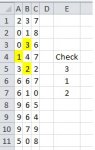
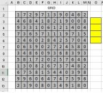
Hi. I am new here and I have been trying to figure out how to get a spreadsheet to do what I need it to, but have not found the exact way to get it done. I have a 10X10 grid of random numbers. What I want to happen is I want a formula encompassing the entire grid, and highlight only the cells that are adjacent to each other if all 3 numbers are there. For example, I included a smaller scale image. I have a grid of numbers and only want the 312 to highlight, but only if the cells are adjacent to each other. I don't want it to highlight all the 3's 1's and 2's. Only if all 3 are there.

Think of it like a wordsearch puzzle. Does this make any sense and can anyone help?

Thanks

 

[DanteAmor]

Hi and welcome to MrExcel.

Using your example as a base, create 3 conditional formatting rules:
Rule 1:
Formula:
=AND(COUNTIF($A1:A1,$F$5)=1,A1=$F$5,MATCH($F$6,$A2:$C2,0),MATCH($F$7,$A3:$C3,0))
Applies to:
=$A$1:$C$10

Rule 2:
Formula:
=AND(COUNTIF($A2:A2,$F$6)=1,A2=$F$6,MATCH($F$5,$A1:$C1,0),MATCH($F$7,$A3:$C3,0))
Applies to:
=$A$2:$C$10

Rule 3:
Formula:
=AND(COUNTIF($A3:A3,$F$7)=1,A3=$F$7,MATCH($F$5,$A1:$C1,0),MATCH($F$6,$A2:$C2,0))
Applies to:
=$A$3:$C$10

 

[JLEMS]

Thank you, I will try and see what the formula is trying to say. I included a snip of the actual grid I am trying to service. I am also looking to expand it later on into have a 4th number as well. I am also going to need to expand the Applies to area to a few other grids on the chart.

 

[DanteAmor]

Thank you, I will try and see what the formula is trying to say. I included a snip of the actual grid I am trying to service. I am also looking to expand it later on into have a 4th number as well. I am also going to need to expand the Applies to area to a few other grids on the chart.

Did you try the formulas in the first example?

 

[JLEMS]

I did, but they are changing themselves to something different and not highlighting. I was going to try and see why

 

[JLEMS]

=AND(COUNTIF($A1048572:XFA1048572,$F$7)=1,XFA1048572=$F$7,MATCH($F$5,$A1048570:$C1048570,0),MATCH($F$6,$A1048571:$C1048571,0))

 

[DanteAmor]

=AND(COUNTIF($A1048572:XFA1048572,$F$7)=1,XFA1048572=$F$7,MATCH($F$5,$A1048570:$C1048570,0),MATCH($F$6,$A1048571:$C1048571,0))

Set this again:
=AND(COUNTIF($A3:A3,$F$7)=1,A3=$F$7,MATCH($F$5,$A1:$C1,0),MATCH($F$6,$A2:$C2,0))

Repeat for the other formulas until the ranges don't change.

 

[JLEMS]

It looks like the formula is sticking now. It highlighted a 0 but one 1

 

[DanteAmor]

Check the range to apply, it is different in each formula.

Formula:
=AND(COUNTIF($A1:A1,$F$5)=1,A1=$F$5,MATCH($F$6,$A2:$C2,0),MATCH($F$7,$A3:$C3,0))
Applies to:
=$A$1:$C$10

Rule 2:
Formula:
=AND(COUNTIF($A2:A2,$F$6)=1,A2=$F$6,MATCH($F$5,$A1:$C1,0),MATCH($F$7,$A3:$C3,0))
Applies to:
=$A$2:$C$10

Rule 3:
Formula:
=AND(COUNTIF($A3:A3,$F$7)=1,A3=$F$7,MATCH($F$5,$A1:$C1,0),MATCH($F$6,$A2:$C2,0))
Applies to:
=$A$3:$C$10

 

[JLEMS]

It's highlighting, but it's highlighting random numbers