Highlight times that are equal to or later than

[alexfooty]

I will do my best to try to explain my problem.

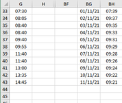
In Col G I have a list of times (hh:mm) that vary each day and also the number of rows may vary.
In Col BG I have a list of dates with a corresponding time in Col BH.

I would like to highlight any times in col G that are equal to, or later than, the time corresponding to today’s date in Col BH

In the following example, If today’s date was 05/11/2021, the corresponding time in Col BH would be 09:31. So any times equal to or later than that would be highlighted in Col G

I hope someone understands this - any help would be greatly appreciated.

 

[alexfooty]

etaf
One or two discrepancies occasionally crop up.
In the example below the time for the conditional formatting to kick in is 16:35 so anything equal to or later should be shaded.

Any ideas as to why this might happen?

 

[etaf]

can you post more of the spreadsheet - the lookup section columns
works for me

Book7
	A	B	C	D
1
2	10:03:00		10/30/21
3	16:21:00		10/31/21
4	16:22:00		11/1/21	11:00:00
5	16:23:00		11/2/21	16:35:00
6	16:24:00
7	16:25:00
8	16:26:00
9	16:27:00
10	16:28:00
11	16:29:00
12	16:30:00
13	16:31:00
14	16:32:00
15	16:33:00
16	16:34:00
17	16:35:00
18	16:36:00
19	16:37:00
20	16:38:00
21	16:39:00
Sheet1

Cells with Conditional Formatting
Cell	Condition		Cell Format	Stop If True
A2:A21	Expression	=A2>=(INDEX($D$2:$D$5,MATCH(TODAY(),$C$2:$C$5,0)))	text	NO

 

[alexfooty]

Cond Format formula =I3>=(INDEX($D3:$D$428,MATCH(TODAY(),$C$3:$C$428,0)))

 

[etaf]

change the format of the times to general for D & I

 

[etaf]

did you select the range I3 or I2 - remember the conditional formatting starts at the cell selected
so if you selected I2:I100
But the formula says I3

then stepping through the cond format
it will look at the cell I2 and then use the formula to test
in this case
is I3 > = which I3 is , but because its looking at i2 - it colours I2

the first row of the range selected, needs to also be in the formula

 

[alexfooty]

If I change the format of D & I to General - I need Col I to show as hh:mm
I selected I3 as the start of the cond format - there is no cond format formula that refers to cell I2

 

[etaf]

ok,
i was only suggesting change the format to see here , not forever, just so we know whats going on and if text or a number
the format does not matter , so you can set for whatever you want to see , BUT only ask to do this just during analysis

So you have selected I3:I??? in conditional formatting
and then using

=I3>=(INDEX($D3:$D$428,MATCH(TODAY(),$C$3:$C$428,0)))

I think you would need to add the spreadsheet here using XL2BB or via a share, like dropbox/onedrive
So i can see what I make of the sample sheet you have setup

 

[alexfooty]

All now seems well. I re-arranged all the columns to match yours (Cols A, C & D) and used the same cond format formula that you used.
This eliminated any of the previous discrepancies.

So I then rearranged the columns back to were I wanted them and re-typed the new references in cond format.
And lo and behold - no discrepancies!!!

I even changed the formula to give me a date next April - checked all my figures and all correct.
Sorry to mess you about etaf and thanks again. Your knowledge and patience knows no bounds.

 

[etaf]

Sorry to mess you about etaf and thanks again

No problem at all
You are very welcome